Constrained Maximum Entropy Modeling of Covid Epidemic
Author
Duncan Foley
Title
Constrained Maximum Entropy Modeling of Covid Epidemic
Description
Documentation and programs for estimating key parameters related to Covid Epidemic from time series data.
Category
Working Material
Keywords
Constrained maximum entropy, Covid epidemic
URL
http://www.notebookarchive.org/2020-11-53br6ow/
DOI
https://notebookarchive.org/2020-11-53br6ow
Date Added
2020-11-11
Date Last Modified
2020-11-11
File Size
7.06 megabytes
Supplements
Rights
CC BY 4.0

Covid epidemic analysis through constrained maximum entropy modeling
Covid epidemic analysis through constrained maximum entropy modeling
Duncan K. Foley
Epidemic modeling
Epidemic modeling
SIR Model
SIR Model
On a given day of an epidemic , let ≥0 be the proportion of a population uninfected and therefore susceptible, ≥0 the proportion of the population infected and infectious, and =1-(+) the proportion of the population either recovered or died, and therefore unsusceptible. is the number of days over which the model tracks the epidemic, starting from day .
t=1,…,T
S
t
F
t
R
t
S
t
F
t
T
1
Let and be the reported number of the population of reported newly infected and dying on day .
x
t
z
t
t
These variables follow the deterministic laws:
S
t+1
S
t
r
t
I
t
I
t+1
I
t
r
t
S
t
I
t
R
t+1
R
t
I
t
x
t
r
t
S
t
I
t
z
t
I
t
(
1
)Here is the infection rate for an encounter between a susceptible and infected person given the pattern of social behavior at day , and are the recovery and death rates for infections, which apply uniformly to the current infected population.
r
t
t
m
d
The number of new cases, , is proportional to the infection rate at day multiplied by the number of infected multiplied by the number of uninfected susceptibles, which is also the number of additional infections on day . The number of infected on day is the number of infected on day less those who die or recover, plus the number of new infections. Hospitalizations, deaths and recoveries are equal to the sum of the corresponding rates over past infections. The model estimates the extent of the infections on days , , the initial proportion of the population susceptible, infected, and removed through resistance to infection, and the parameters .
x
t
t
t+1
t+1
t
t=1,…T
I
t
m,d,
r
t
Data consist of daily observations of new “confirmed” cases for the last days, , and deaths, .
T
x={,…,}
x
1
x
T
z={,…,}
z
1
z
T
Probabilities and maximum entropy
Probabilities and maximum entropy
Constrained maximum entropy model
Constrained maximum entropy model
Since the data relevant to this model take the form of specific counts of infections and deaths, rather than expectations, from an Info-metric point of view the analysis of this system requires the “general” form of the info-metric constrained maximum entropy system, which includes error terms on the constraints.
The idea is that changing social behavior to depress below a reference level requires social “force” similar to the physical force depressing a spring, and results in a potential energy , which trades off against the entropy of the frequency distributions of error terms on the observed data. We also want to penalize the variation in using a Hodrick-Prescott-like square of second differences. We also will specify an underreporting rate , which adjusts actual infections to reported infections, with an exponential penalty weighted by a parameter .
r
t
r
0
1
2
2
k(-)
r
0
r
t
r
t
b≥0
α
Max
S
t
I
t
r
t
T
∑
t=1
1
2
2
k(-)
r
0
r
t
u
t
u
t
w
t
w
t
T-1
∑
t=2
2
((-)-(-))
r
t+1
r
t
r
t
r
t-1
2
β(r[0]-)
r
S
t+1
S
t
r
t
F
t
r
0
r
t
F
t+1
I
t
r
t
S
t
F
t
x
t
pop
r
t
S
t
I
t
ϵ
t
r
t
S
t
F
t
u
t
z
t
pop
I
t
χ
t
F
t
v
t
(
2
)u
t
v
t
M
M
q,s
We know , for days from the data, and want to infer the history of the epidemic, the matrix , along with the matrices ,, the dimensional vector , parameters , conditional on the parameters , and the population, subject to the constraints (
x
t
z
t
T
T×2
{,}
S
t
F
t
T×M
u
t
v
t
T
r
t
m,d,b,
r
0
k,α,γ
2
).The international data does not report hospitalizations, which are eliminated from the simulations.
Dynamic analysis
Dynamic analysis
Mathematica code
Mathematica code
Protection from corrupt outliers
Protection from corrupt outliers
Mathematica simulation programs
Mathematica simulation programs
In[]:=
ClearAll[EpidemicCMEObjConst];EpidemicCMEObjConst[opts:OptionsPattern[{EpidemicCME}]][data:{country_,datelabel_,pop_,popwt_,totinf_,infwt_,{x_List,z_List}}]:=WithT=Length[x],datamean=Mean/@//N,errormax=OptionValue@supportwidthMax[#,$MachineEpsilon]&/@StandardDeviation/@//N,qq=Tablej,j,-#,#,&/@OptionValue@supportwidthMax[#,$MachineEpsilon]&/@StandardDeviation/@//N,-OptionValue@kPlus@@-OptionValue@γPlus@@-OptionValue@αb+infentropy[Flatten@Array[u,{T,OptionValue@M}]]+infentropy[Flatten@Array[v,{T,OptionValue@M}]],Thread[0≤Flatten[{Array[S,{T+1}],Array[F,{T+1}],Array[r,{T+2},{0}],Array[u,{T,OptionValue@M}],Array[v,{T,OptionValue@M}],m,d}]],Thread[Flatten[{Array[S,{T+1}],Array[F,{T+1}]}]≤1],Thread[Flatten[{Array[r,{T+1}]}]≤r[0]],Thread[Total/@Array[u,{T,OptionValue@M}]1],Thread[Total/@Array[v,{T,OptionValue@M}]1],Rest@Array[S,{T+1}](Most@Array[S,{T+1}]-Most@(Array[S,{T+1}]Array[r,{T+1}]Array[F,{T+1}])),Rest@Array[F,{T+1}]Most@((1-(d+m))Array[F,{T+1}]+(Array[r,{T+1}]Array[F,{T+1}]Array[S,{T+1}])),SelectThreadbArray[r,{T}]Array[F,{T}]Array[S,{T}]+Array[u,{T,OptionValue@M}].qq[[1]],#[[1]]≥0&&Abs[datamean[[1]]-#[[1]]]≤errormax[[1]]&,SelectThreaddArray[F,{T}]+Array[v,{T,OptionValue@M}].qq[[2]],#[[1]]≥0&&Abs[datamean[[2]]-#[[1]]]≤errormax[[2]]&,OptionValue@addedconstraints
Select[#≥0&]/@{x,z}
pop
Select[#≥0&]/@{x,z}
pop
2#
OptionValue@M-1
Select[#≥0&]/@{x,z}
pop
1
2
2
(r[0]-Array[r,{T+1}])
2
Differences[Array[r,{T+1}],2]
x
pop
z
pop
In[]:=
EpidemicCMEObjConst[addedconstraints->{S[1]≥.9,m≤.3}][{"NYC","March-May2020",8,1,1,Transpose[NYCData][[{2,4},2;;]]}]
6
10
In[]:=
Clear[EpidemicCME,infentropy];infentropy[p:{__}]:=Plus@@(Cases[p,Except[0]]/.x_->-xLog[x]);Options[EpidemicCME]=k,γ,α0,addedconstraints{},supportwidth3,M3;EpidemicCME[opts:OptionsPattern[{EpidemicCME,FindMaximum}]][data:{country_,datelabel_,pop_,popwt_,totinf_,infwt_,{x_List,z_List}}]:={(#[[1]]OptionValue[#[[1]]])&/@Options[EpidemicCME],FindMaximum[EpidemicCMEObjConst[FilterRules[{opts},{Options[EpidemicCME]}]][data],Evaluate@Flatten[{{m,d,b,r[0]},Array[r,{Length[x]+1}],Array[S,{Length[x]+1}],Array[F,{Length[x]+1}],Array[u,{Length[x],OptionValue@M}],Array[v,{Length[x],OptionValue@M}]}]],country,datelabel,pop,popwt,totinf,infwt,{x,z}}
1
10
3
10
NYC Data Epidemic to August 23, 2020
NYC Data Epidemic to August 23, 2020
Import cases, hospitalizations, death data:
In[]:=
Clear[NYCData];(NYCData=Import["https://github.com/nychealth/coronavirus-data/raw/master/case-hosp-death.csv"]);
In[]:=
NYCData[[1;;10]]//Shallow
Out[]//Shallow=
{{DATE_OF_INTEREST,CASE_COUNT,HOSPITALIZED_COUNT,DEATH_COUNT,CASE_COUNT_7DAY_AVG,INCOMPLETE},{02/29/2020,1,0,0,,},{03/03/2020,1,1,0,,},{03/04/2020,5,2,0,,},{03/05/2020,3,8,0,,},{03/06/2020,8,5,0,,},{03/07/2020,7,6,0,,},{03/08/2020,21,15,0,7,},{03/09/2020,57,30,0,15,},{03/10/2020,70,49,0,24,}}
NYCTest
NYCTest
In[]:=
Clear[NYCTest];(NYCTest=EpidemicCME[][{"NYC","March-October 22 2020",8,1,Total@Transpose[NYCData][[4,2;;]],1,Transpose[NYCData][[{2,4},2;;]]}]);//Timing
6
10
Out[]=
{4.5749,Null}
In[]:=
NYCTest[[2,2]]//Shallow
Out[]//Shallow=
{m0.148074,d0.000656522,b0.0477112,r[1]0.359784,r[1]0.358972,r[1]0.359083,r[1]0.359193,r[1]0.359301,r[1]0.359405,r[1]0.359502,2112}
Simulations
Simulations
Simulation summary, plot, and report programs
Simulation summary, plot, and report programs
Report and plot simulations:
In[]:=
Clear[EpidemicCMESummary];Options[EpidemicCMESummary]=reportparams,,,1-,b,fitstatsFalse;EpidemicCMESummary[opts:OptionsPattern[{ListPlot,EpidemicCME,EpidemicCMESummary}]][simlong:{options_,{score_,simul_List},country_,datelabel_,pop_,popwt_,totinf_,infwt_,{x_List,z_List}}]:=With{T=Length[x],M=M/.options,sim=Flatten@{options,simul}},Columncountry,datelabel,Row[Evaluate[Flatten[{{#(#/.sim)}&/@OptionValue@reportparams,{populationpop,popweightpopwt,totinfectionstotinf,infweightinfwt}}]],", "],Row[options,", "],IfOptionValue@fitstats,Row"logfit"-kPlus@@-γPlus@@-αb+infentropy[Flatten@Array[u,{T,M}]]+infentropy[Flatten@Array[v,{T,M}]]-2TLog[M]/.sim,"resistance"->-kPlus@@/.sim,"smoothing"->(-γPlus@@)/.sim,"reporting"->(-αb)/.sim,"entropy deficit"->(infentropy[Flatten@Array[u,{T,M}]]+infentropy[Flatten@Array[v,{T,M}]]-2TLog[M])/.sim,", ","",Center//NumberForm[#,{12,3}]&
1
m+d
d
m+d
r[0]
m+d
m+d
r[0]
1
2
2
(r[0]-Array[r,{T+1}])
2
Differences[Array[r,{T+1}],2]
1
2
2
(r[0]-Array[r,{T+1}])
2
Differences[Array[r,{T+1}],2]
In[]:=
EpidemicCMESummary[fitstatsTrue][EpidemicCME[][{"NYC","March-September 2020",8,1,Total@Transpose[NYCData][[4,2;;]],1,Transpose[NYCData][[{2,4},2;;]]}]]
6
10
Out[]//NumberForm=
NYC |
March-September 2020 |
1 d+m d d+m r[0] d+m d+m r[0] |
k 1 10 |
logfit-1.791, resistance-0.074, smoothing-0.031, reporting0.000, entropy deficit-1.686 |
Increase penalty on reporting:
In[]:=
EpidemicCMESummary[fitstatsTrue][EpidemicCME[α100][{"NYC","March-September 2020",8,1,Total@Transpose[NYCData][[4,2;;]],1,Transpose[NYCData][[{2,4},2;;]]}]]
6
10
Out[]//NumberForm=
NYC |
March-September 2020 |
1 d+m d d+m r[0] d+m d+m r[0] |
k 1 10 |
logfit-4.655, resistance-0.068, smoothing-0.043, reporting-2.384, entropy deficit-2.160 |
In[]:=
Clear[EpidemicCMEPlot];Options[EpidemicCMEPlot]={InfRiskScale};EpidemicCMEPlot[opts:OptionsPattern[{ListPlot,EpidemicCMEPlot,EpidemicCME,EpidemicCMESummary}]][simlong:{options_,{score_,simul_List},country_,datelabel_,pop_,popwt_,totinf_,infwt_,{x_List,z_List}}]:=With{T=Length[x],M=M/.options,sim=Flatten@{options,simul},datalabel=country<>"\n"<>datelabel},Grid@ListLogPlot/.sim,(Array[S,{T}]Array[r,{T}]Array[F,{T}])/.sim,(bArray[S,{T}]Array[r,{T}]Array[F,{T}])/.sim,-bArray[S,{T}]Array[r,{T}]Array[F,{T}]/.sim,JoinedTrue,AxesLabel{"Day","Log Infections"},PlotStyle{{Blue},{Orange},{Red},{Opacity[.5],Green}},PlotLegendsPlaced[{"New Infections","Model Reported New Infections","Model New Infections","Error"},Below],PlotLabeldatalabel<>"\nInfections",FilterRules[{opts},Options[ListPlot]],PlotRange->All,ListPlot/.sim,(dArray[F,{T}])/.sim,-dArray[F,{T}]/.sim,JoinedTrue,AxesLabel{"Day","Deaths"},PlotStyle{{Blue},{Orange},{Opacity[.5],Green}},PlotLegendsPlaced[{"Deaths","Model Deaths","Error"},Below],PlotLabeldatalabel<>"\nDeaths",FilterRules[{opts},Options[ListPlot]],PlotRange->All,ListPlotTable,{T},,,OptionValue@InfRiskScaleArray[r,{T}]Array[F,{T}],Table[1,{T}]/.sim,PlotStyle{{Orange},{Red},{Blue},{Green},{Thickness[Large],{Dashed,Gray}}},JoinedTrue,AxesLabel{"Day","Epidemic"},PlotLegendsPlaced"Initial Infection Factor, ","Infection Factor, ","Infection Rate, ","Infection Risk, x "<>ToString[OptionValue@InfRiskScale](*,"Stability Threshold, 1"*),Below,PlotLabeldatalabel<>"\nInfection Rates",FilterRules[{opts},Options[ListPlot]],PlotRangeAll,ListPlot[{Array[F,{T}],1-Array[S,{T}]-Array[F,{T}]}/.sim,JoinedTrue,AxesLabel{"Day","Epidemic"},PlotLegendsPlaced[{"Infected","Removed"},Below],PlotLabeldatalabel<>"\nInfected, Removed",FilterRules[{opts},Options[ListPlot]]]
2
10
x
pop
x
pop
z
pop
z
pop
r[0]
m+d
Array[r,{T}]Array[S,{T}]
m+d
Array[r,{T}]
m+d
r
0
m+d
r
t
S
t
m+d
r
t
m+d
r
t
F
t
In[]:=
EpidemicCMEPlot[ImageSizeMedium][NYCTest]
In[]:=
Clear[EpidemicCMEReport];EpidemicCMEReport[opts:OptionsPattern[{ListPlot,EpidemicCME,EpidemicCMESummary}]][simlong_]:=Column@{EpidemicCMESummary[FilterRules[{opts},Options[EpidemicCMESummary]]][simlong],EpidemicCMEPlot[FilterRules[{opts},{Options[EpidemicCMESummary],Options[ListPlot]}]][simlong]}
In[]:=
EpidemicCMEReport[ImageSizeMedium,fitstatsTrue][EpidemicCME[α0][{"NYC","March-September 2020",8,1,Total@Transpose[NYCData][[4,2;;]],1,Transpose[NYCData][[{2,4},2;;]]}]]
6
10
Out[]=
| ||||||||||||||||||||||||||||||||||||||||||||||
|


In[]:=
EpidemicCMEReport[ImageSizeMedium,fitstatsTrue][EpidemicCME[k.01][{"NYC","March-October 22 2020",8,1,Total@Transpose[NYCData][[4,2;;]],1,Transpose[NYCData][[{2,4},2;;]]}]]
6
10
Out[]=
| ||||||||||||||||||||||||||||||||||||||||||||||
|


Try bigger :
k
In[]:=
EpidemicCMEReport[ImageSizeMedium,fitstatsTrue][EpidemicCME[k1][{"NYC","March-October 22 2020",8,1,Total@Transpose[NYCData][[4,2;;]],1,Transpose[NYCData][[{2,4},2;;]]}]]
6
10
Out[]=
| ||||||||||||||||||||||||||||||||||||||||||||||
|


Compare to constraining .
b=1
In[]:=
EpidemicCMEReport[ImageSizeMedium,fitstatsTrue][EpidemicCME[addedconstraints{b1}][{"NYC","March-October 22 2020",8,1,Total@Transpose[NYCData][[4,2;;]],1,Transpose[NYCData][[{2,4},2;;]]}]]
6
10
Out[]=
| ||||||||||||||||||||||||||||||||||||||||||||||
|


The ratio of posterior probability is:
In[]:=
-1.805-(-2.054)
Out[]=
0.249
In[]:=
Exp[%]
Out[]=
1.28274
Compare to constraining .
b≥.08
In[]:=
EpidemicCMEReport[ImageSizeMedium,fitstatsTrue][EpidemicCME[addedconstraints{b≥.08}][{"NYC","March-October 22 2020",8,1,Total@Transpose[NYCData][[4,2;;]],1,Transpose[NYCData][[{2,4},2;;]]}]]
6
10
Out[]=
| ||||||||||||||||||||||||||||||||||||||||||||||
|


In[]:=
EpidemicCMEReport[ImageSizeMedium,fitstatsTrue][EpidemicCME[addedconstraints{b≥.2}][{"NYC","March-October 22 2020",8,1,Total@Transpose[NYCData][[4,2;;]],1,Transpose[NYCData][[{2,4},2;;]]}]]
6
10
Out[]=
| ||||||||||||||||||||||||||||||||||||||||||||||
|


The difference between unconstrained and log fits is:
b≥.08
In[]:=
-1.876-(-2.12)
Out[]=
0.244
The ratio of the posterior probabilities is:
In[]:=
Exp[%]
Out[]=
1.27634
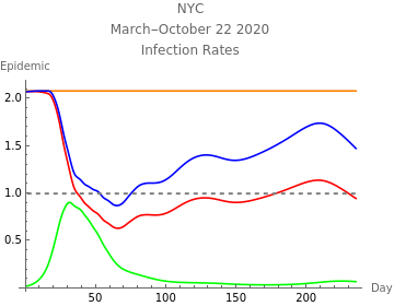
The first line documents the country or region and dates of the analysis. The second line documents the specific options under which the analysis was run. The critical parameter is , which controls the cost of changing the , which has been chosen by trial and error to produce smooth plots with significant response of the daily infection rate to changes in social behavior.
k
r
t
The next line reports the estimated parameters, , the proportion of the infected recovering per day, , the mortality rate for the infected, , the base infection rate, , the mean length of the disease, , the infection rate adjusted for the mean length of the disease, which is comparable to widely quoted infection rates, and , the herd immunity threshold, which is the proportion of the population that must be immune for herd immunity.
m
d
r[0]
1
m+d
r[1]
m+d
1-
d+m
r[1]
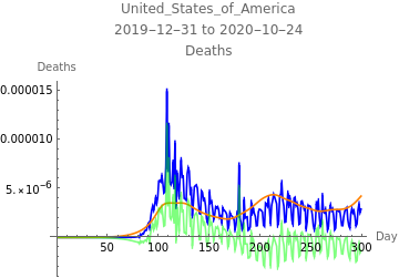
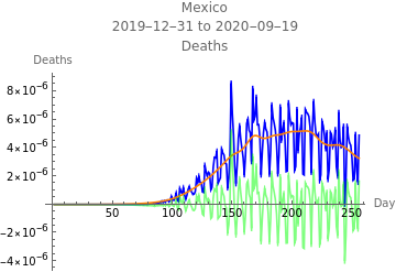
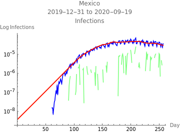
The first plot shows new infections per capita as reported in the data in blue, the model fit to infections in orange, the model fit to reported infections taking account of the reporting rate, and errors in green. The second plot shows deaths per capita as reported in the data in blue, the model fit to deaths in orange, and errors in green.
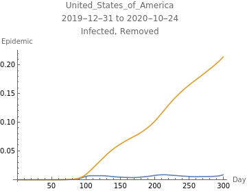
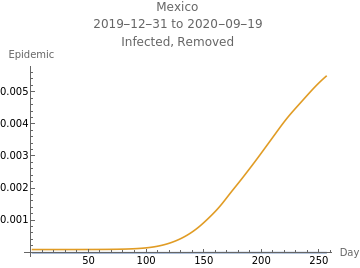
The third plot shows the estimated initial adjusted infection rate as a horizontal orange line, the estimated daily adjustejd infection rates in blue, the product , which is the inherent daily rate of increase of the infection, in red, the stability threshold,1, as a horizontal dashed line, and the daily risk of infection, , multiplied by . When the susceptible population is very close to 100%, ≈ and the plotted curves lie directly over each other. The lower right plot shows the daily proportion of infected in blue, and removed through recovery or death in orange.
r
1
m+d
r
t
m+d
r
t
S
t
m+d
r
t
I
t
3
10
r
t
m+d
r
t
S
t
m+d
Modify EpidemicCME for access to Global data
Modify EpidemicCME for access to Global data
Mathematica programs
Mathematica programs
International epidemic data
International epidemic data
Global data from European CDPC:
In[]:=
Clear[GlobalData];(GlobalData=Import["https://opendata.ecdc.europa.eu/covid19/casedistribution/csv"])//Dimensions
Out[]=
{51043,12}
The statistics provided by the European CDC dataset are:
In[]:=
GlobalData[[1]]
Out[]=
{dateRep,day,month,year,cases,deaths,countriesAndTerritories,geoId,countryterritoryCode,popData2019,continentExp,Cumulative_number_for_14_days_of_COVID-19_cases_per_100000}
The countries covered are:
In[]:=
(countrynames=Union[Select[Rest@GlobalData,And@@(NumberQ/@#[[{"day","month","year","cases","deaths","popData2019"}/.Flatten@MapIndexed[{#1#2[[1]]}&,First@GlobalData]]])&][[All,7]]])
Out[]=
{Afghanistan,Albania,Algeria,Andorra,Angola,Anguilla,Antigua_and_Barbuda,Argentina,Armenia,Aruba,Australia,Austria,Azerbaijan,Bahamas,Bahrain,Bangladesh,Barbados,Belarus,Belgium,Belize,Benin,Bermuda,Bhutan,Bolivia,Bonaire, Saint Eustatius and Saba,Bosnia_and_Herzegovina,Botswana,Brazil,British_Virgin_Islands,Brunei_Darussalam,Bulgaria,Burkina_Faso,Burundi,Cambodia,Cameroon,Canada,Cape_Verde,Cayman_Islands,Central_African_Republic,Chad,Chile,China,Colombia,Comoros,Congo,Costa_Rica,Cote_dIvoire,Croatia,Cuba,Curaçao,Cyprus,Czechia,Democratic_Republic_of_the_Congo,Denmark,Djibouti,Dominica,Dominican_Republic,Ecuador,Egypt,El_Salvador,Equatorial_Guinea,Eritrea,Estonia,Eswatini,Ethiopia,Falkland_Islands_(Malvinas),Faroe_Islands,Fiji,Finland,France,French_Polynesia,Gabon,Gambia,Georgia,Germany,Ghana,Gibraltar,Greece,Greenland,Grenada,Guam,Guatemala,Guernsey,Guinea,Guinea_Bissau,Guyana,Haiti,Holy_See,Honduras,Hungary,Iceland,India,Indonesia,Iran,Iraq,Ireland,Isle_of_Man,Israel,Italy,Jamaica,Japan,Jersey,Jordan,Kazakhstan,Kenya,Kosovo,Kuwait,Kyrgyzstan,Laos,Latvia,Lebanon,Lesotho,Liberia,Libya,Liechtenstein,Lithuania,Luxembourg,Madagascar,Malawi,Malaysia,Maldives,Mali,Malta,Mauritania,Mauritius,Mexico,Moldova,Monaco,Mongolia,Montenegro,Montserrat,Morocco,Mozambique,Myanmar,Namibia,Nepal,Netherlands,New_Caledonia,New_Zealand,Nicaragua,Niger,Nigeria,Northern_Mariana_Islands,North_Macedonia,Norway,Oman,Pakistan,Palestine,Panama,Papua_New_Guinea,Paraguay,Peru,Philippines,Poland,Portugal,Puerto_Rico,Qatar,Romania,Russia,Rwanda,Saint_Kitts_and_Nevis,Saint_Lucia,Saint_Vincent_and_the_Grenadines,San_Marino,Sao_Tome_and_Principe,Saudi_Arabia,Senegal,Serbia,Seychelles,Sierra_Leone,Singapore,Sint_Maarten,Slovakia,Slovenia,Solomon_Islands,Somalia,South_Africa,South_Korea,South_Sudan,Spain,Sri_Lanka,Sudan,Suriname,Sweden,Switzerland,Syria,Taiwan,Tajikistan,Thailand,Timor_Leste,Togo,Trinidad_and_Tobago,Tunisia,Turkey,Turks_and_Caicos_islands,Uganda,Ukraine,United_Arab_Emirates,United_Kingdom,United_Republic_of_Tanzania,United_States_of_America,United_States_Virgin_Islands,Uruguay,Uzbekistan,Venezuela,Vietnam,Western_Sahara,Yemen,Zambia,Zimbabwe}
In[]:=
Length@countrynames
Out[]=
209
Sample simulation -- U.S.
Sample simulation -- U.S.
In[]:=
EpidemicCMEReport[fitstatsTrue,ImageSizeMedium][EpidemicCME[][FirstCase[EpidemicCMEData[][GlobalData],{"United_States_of_America",___}]]]
Out[]=
| ||||||||||||||||||||||||||||||||||||||||||||||
|


In[]:=
EpidemicCMEReport[fitstatsTrue,ImageSizeMedium][EpidemicCME[addedconstraints{b≥.08}][FirstCase[EpidemicCMEData[][GlobalData],{"United_States_of_America",___}]]]
Out[]=
| ||||||||||||||||||||||||||||||||||||||||||||||
|


In[]:=
EpidemicCMEReport[fitstatsTrue,ImageSizeMedium][EpidemicCME[k.01][FirstCase[EpidemicCMEData[][GlobalData],{"United_States_of_America",___}]]]
Out[]=
| ||||||||||||||||||||||||||||||||||||||||||||||
|


In[]:=
EpidemicCMEReport[fitstatsTrue,ImageSizeMedium][EpidemicCME[k1][FirstCase[EpidemicCMEData[][GlobalData],{"United_States_of_America",___}]]]
Out[]=
| ||||||||||||||||||||||||||||||||||||||||||||||
|


The improvement in log fit between unconstrained and unconstrained is about .4, which corresponds to a ratio of posterior probability of around 1.5:
k=.1
k=1
In[]:=
diff=-13.479-(-14.002)
Out[]=
0.523
In[]:=
Exp[diff]
Out[]=
1.68708
Mean and standard deviation with and without weighting
Mean and standard deviation with and without weighting
In[]:=
Clear[CMEStats];CMEStats[simulset_][stats_]:=Column[{TableForm[With[{stat=#},{stat,#[[1]],#[[2]]}&@({Mean[#],StandardDeviation[#]}&/@{(stat/.simulset[[All,1,1,3,1]]),(WeightedData@@Transpose[{stat,infweight}/.simulset[[All,1,1,3,1]]])})]&/@stats,TableHeadings{None,{"Stat","Unweighted\nMean, SD","Infection Weighted\nMean, SD"}},TableDirections{Column,Row,Row}],simulset[[1,1,1,4,1]]},Center]
International sample ranked by infection sizes
International sample ranked by infection sizes
In[]:=
TableForm[infwtsummary=Transpose@Flatten[{#,{FoldList[Plus,#[[3]]]}},1]&@Transpose@Sort[EpidemicCMEData[][GlobalData][[All,{1,5,6}]],#1[[2]]≥#2[[2]]&],TableHeadings{None,{"Country","TotInf","InfWeight","CumInfWeight"}}]
Unconstrained estimates of epidemics larger than 410 infections
Unconstrained estimates of epidemics larger than infections
4
10
In[]:=
(EpidemicCMESurvey1=Quiet@TimeConstrained[Check[EpidemicCMESummary[][EpidemicCME[][#]],#[[1]]<>" error"],30,#[[1]]<>" timeout"]&/@Select[EpidemicCMEData[][GlobalData],#[[5]]≥&])//Dimensions//Timing
4
10
Out[]=
{1077.7,{110}}
In[]:=
Select[EpidemicCMESurvey1,Length[#]==0&]
Out[]=
{Algeria error,Bahrain error,Belarus error,Cote_dIvoire timeout,El_Salvador timeout,Ethiopia error,Guatemala timeout,India timeout,Indonesia error,Kenya timeout,Libya error,Maldives error,Nepal error,Nigeria error,Singapore timeout,Slovakia error,Uganda error,United_Arab_Emirates timeout,Zambia timeout}
In[]:=
(validSurvey1=Select[EpidemicCMESurvey1,Length[#]>0&])//Dimensions
Out[]=
{91}
In[]:=
validSurvey1[[All,1,1,3,1]]//Dimensions
Out[]=
{91,9}
In[]:=
validSurvey1[[1,1,1,3,1]]
Out[]=
25.2519,0.118078,2.56848,1-0.610665,b3.55736,population38041757,popweight0.00495989,totinfections40687.,infweight0.000962344
1
d+m
d
d+m
r[0]
d+m
d+m
r[0]
Weighted quantile statistics
Weighted quantile statistics
In[]:=
Clear[SurveyDist];SurveyDist[survey_][stat_]:=SurveyDist[survey][stats]=EmpiricalDistribution[(infweight/.survey[[All,1,1,3,1]])(stat/.survey[[All,1,1,3,1]])]
In[]:=
Clear[CMEQuantStats];CMEQuantStats[simulset_][stats_]:=Column[{TableForm[{#,Median[SurveyDist[simulset][#]],Quantile[SurveyDist[simulset][#],{.25,.75}]}&/@stats,TableHeadings->{None,{"Stat","Infection Weighted\nMedian","Interquartile Range"}},TableDirections->{Column,Row,Column}],simulset[[1,1,1,4,1]]},Center]//NumberForm[#,{6,3}]&
Statistics
Statistics
The computation of summary statistics requires weighting the individual country outcomes. The most relevant weighting would seem to be by infections, since the model is fitting infection data. The
In[]:=
CMEQuantStats[validSurvey1],,,1-,b
1
m+d
d
m+d
r[0]
m+d
m+d
r[0]
Out[]//NumberForm=
| ||||||||||||||||||||||||||||
k 1 10 |
Histograms
Histograms
To get the weighted histogram:
In[]:=
(inflength=HistogramDistribution[WeightedData@@Transpose[Select[{1/(m+d),infweight}/.validSurvey1[[All,1,1,3,1]],#[[1]]<50&]],{1}])
Out[]=
DataDistribution
 |
|
In[]:=
Plot[CDF[inflength,x],{x,0,50}]
Out[]=
In[]:=
Mean[inflength]
Out[]=
6.77224
In[]:=
Histogram[WeightedData@@Transpose[{1/(m+d),infweight}/.Select[validSurvey1,(((1/(m+d))/.#[[1,1,3,1]])≤50)&][[All,1,1,3,1]]],{1}]
Out[]=
In[]:=
Sort[{#[[1,1,1]],1/(m+d)/.#[[1,1,3,1]],infweight/.#[[1,1,3,1]]}&/@Select[validSurvey1,(((1/(m+d))/.#[[1,1,3,1]])>50)&],#1[[2]]>#2[[2]]&]//TableForm[#,TableHeadings{None,{"Country","Infection Length","InfWeight"}}]&
Out[]//TableForm=
Country | Infection Length | InfWeight |
Guinea | 1.85176× 7 10 | 0.000275195 |
Kazakhstan | 1.26072× 6 10 | 0.00347647 |
Ecuador | 451090. | 0.00374346 |
Peru | 215944. | 0.0208878 |
Bolivia | 113197. | 0.00332581 |
Puerto_Rico | 12972.4 | 0.00144242 |
Moldova | 9842.25 | 0.00166172 |
Oman | 8946.66 | 0.00264521 |
Ukraine | 6859.77 | 0.00781465 |
Bosnia_and_Herzegovina | 6603.38 | 0.00091045 |
Tunisia | 5893.38 | 0.00111672 |
Argentina | 2418.19 | 0.0252928 |
Cameroon | 346.772 | 0.000510181 |
Tajikistan | 56.6445 | 0.000252962 |
In[]:=
Histogram[WeightedData@@Transpose[{d/(m+d),infweight}/.validSurvey1[[All,1,1,3,1]]],{.001}]
Out[]=
In[]:=
Histogram[WeightedData@@Transpose[{r[0]/(m+d),infweight}/.validSurvey1[[All,1,1,3,1]]],{.1}]
Out[]=
High infection rates:
In[]:=
Sort[{#[[1,1,1]],r[0]/(m+d)/.#[[1,1,3,1]],infweight/.#[[1,1,3,1]]}&/@Select[validSurvey1,(((r[0]/(m+d))/.#[[1,1,3,1]])>4.0)&],#1[[2]]>#2[[2]]&]//TableForm[#,TableHeadings{None,{"Country","Infection Factor","InfWeight"}}]&
Out[]//TableForm=
Country | Infection Factor | InfWeight |
Zambia | 8600.92 | 0.000459129 |
Kazakhstan | 1625.4 | 0.00451902 |
Philippines | 540.113 | 0.00915265 |
Ecuador | 444.11 | 0.00406441 |
Bulgaria | 333.194 | 0.000613383 |
Ukraine | 299.484 | 0.0055491 |
Libya | 261.463 | 0.000865672 |
Bolivia | 219.354 | 0.00425832 |
Peru | 206.711 | 0.0247675 |
Bosnia_and_Herzegovina | 193.52 | 0.00081505 |
Puerto_Rico | 151.514 | 0.00129939 |
Belarus | 6.07875 | 0.00246329 |
Hungary | 5.6262 | 0.000554019 |
Oman | 5.36953 | 0.00300431 |
South_Korea | 5.2742 | 0.000749596 |
Australia | 4.82186 | 0.000879522 |
Low infection rates:
In[]:=
Sort[{#[[1,1,1]],r[0]/(m+d)/.#[[1,1,3,1]],infweight/.#[[1,1,3,1]]}&/@Select[validSurvey1,(((r[0]/(m+d))/.#[[1,1,3,1]])≤1.25)&],#1[[2]]<#2[[2]]&]//TableForm[#,TableHeadings{None,{"Country","Infection Factor","InfWeight"}}]&
Out[]//TableForm=
Country | Infection Factor | InfWeight |
Cameroon | 0.324127 | 0.000667017 |
Mexico | 1.00066 | 0.0225587 |
Sweden | 1.00069 | 0.00288919 |
Colombia | 1.00126 | 0.024573 |
Guatemala | 1.00133 | 0.00276171 |
Brazil | 1.00172 | 0.147188 |
Kyrgyzstan | 1.01193 | 0.00148442 |
North_Macedonia | 1.06427 | 0.000537549 |
Kuwait | 1.10083 | 0.00322615 |
Serbia | 1.12495 | 0.00107258 |
Namibia | 1.15996 | 0.000334213 |
Venezuela | 1.17503 | 0.00213402 |
Pakistan | 1.19666 | 0.00998777 |
In[]:=
Histogram[WeightedData@@Transpose[{1-((m+d)/r[0]),infweight}/.validSurvey1[[All,1,1,3,1]]],{.05}]
Out[]=
Leading cases
Leading cases
In[]:=
Quiet@EpidemicCMEReport[fitstatsTrue][TimeConstrained[Check[EpidemicCME[addedconstraints{1≥b≥.1}][#],#[[1]]<>" error"],30,#[[1]]<>" timeout"]]&/@Cases[Select[EpidemicCMEData[][GlobalData],#[[5]]≥&],{Alternatives@@{"China","India","United_Kingdom","France","Italy","Spain","Germany","Sweden","Russia","Brazil","Mexico"},___}]
4
10
Out[]=
In[]:=
With[{exportdirectory=SystemDialogInput["Directory"]},Export[FileNameJoin[{exportdirectory,#[[1]]<>"Report.pdf"}],Quiet@EpidemicCMEReport[fitstatsTrue][TimeConstrained[Check[EpidemicCME[addedconstraints{1≥b≥.1}][#],#[[1]]<>" error"],30,#[[1]]<>" timeout"]]]&/@Cases[Select[EpidemicCMEData[][GlobalData],#[[5]]≥&],{Alternatives@@{"China","India","United_Kingdom","France","Italy","Spain","Germany","Sweden","Russia","United_States_of_America","Brazil","Mexico"},___}]]
4
10
Out[]=
{/Users/dkf/Dropbox/Active Projects/EpidemicCMEModel/Paper/Figures/BrazilReport.pdf,/Users/dkf/Dropbox/Active Projects/EpidemicCMEModel/Paper/Figures/ChinaReport.pdf,/Users/dkf/Dropbox/Active Projects/EpidemicCMEModel/Paper/Figures/FranceReport.pdf,/Users/dkf/Dropbox/Active Projects/EpidemicCMEModel/Paper/Figures/GermanyReport.pdf,/Users/dkf/Dropbox/Active Projects/EpidemicCMEModel/Paper/Figures/IndiaReport.pdf,/Users/dkf/Dropbox/Active Projects/EpidemicCMEModel/Paper/Figures/ItalyReport.pdf,/Users/dkf/Dropbox/Active Projects/EpidemicCMEModel/Paper/Figures/MexicoReport.pdf,/Users/dkf/Dropbox/Active Projects/EpidemicCMEModel/Paper/Figures/RussiaReport.pdf,/Users/dkf/Dropbox/Active Projects/EpidemicCMEModel/Paper/Figures/SpainReport.pdf,/Users/dkf/Dropbox/Active Projects/EpidemicCMEModel/Paper/Figures/SwedenReport.pdf,/Users/dkf/Dropbox/Active Projects/EpidemicCMEModel/Paper/Figures/United_KingdomReport.pdf,/Users/dkf/Dropbox/Active Projects/EpidemicCMEModel/Paper/Figures/United_States_of_AmericaReport.pdf}
In[]:=
Sort[{#[[1,1,1]],1/(m+d)/.#[[1,1,3,1]],infweight/.#[[1,1,3,1]]}&/@Select[validSurvey1,(((1/(m+d))/.#[[1,1,3,1]])<2)&],#1[[2]]>#2[[2]]&]//TableForm[#,TableHeadings{None,{"Country","Infection Length","InfWeight"}}]&
Out[]//TableForm=
Country | Infection Length | InfWeight |
Morocco | 0.990218 | 0.0022494 |
Libya | 0.359698 | 0.000465027 |
Brazil | 0.18371 | 0.153032 |
Colombia | 0.166623 | 0.023304 |
Kuwait | 0.162733 | 0.0034198 |
United_Arab_Emirates | 0.0755159 | 0.00284203 |
Ecuador | 0.0656664 | 0.00457419 |
Sweden | 0.0560138 | 0.00366315 |
Iraq | 0.0539317 | 0.00878541 |
Mexico | 0.0469961 | 0.0238112 |
India | 0.0359437 | 0.13379 |
Guatemala | 0.0341402 | 0.00289488 |
Palestine | 0.0339348 | 0.00108085 |
El_Salvador | 0.0312577 | 0.00104803 |
United_Kingdom | 0.0272322 | 0.0137964 |
Kyrgyzstan | 0.021323 | 0.0018267 |
Serbia | 0.0203788 | 0.00129738 |
Ghana | 0.017959 | 0.00184262 |
Indonesia | 0.00884723 | 0.0065647 |
Cote_dIvoire | 0.0073122 | 0.000739464 |
Algeria | 0.00600536 | 0.00176811 |
Zambia | 0.00393518 | 0.000470898 |
Nigeria | 0.00212767 | 0.00221966 |
Constraining infection length:
In[]:=
Quiet@EpidemicCMEReport[fitstatsTrue][TimeConstrained[Check[EpidemicCME[addedconstraints{.03≤m+d≤.5,.1≤b≤1}][#],#[[1]]<>" error"],30,#[[1]]<>" timeout"]]&/@Cases[Select[EpidemicCMEData[][GlobalData],#[[5]]≥&],{Alternatives@@{"India","Sweden","Brazil","Mexico"},___}]
4
10
Out[]=
,
,
,
| ||||||||||||||||||||||||||||||||||||||||||||||
|


EpidemicCMESummary[{fitstatsTrue}][India error] |
EpidemicCMEPlot[{fitstatsTrue}][India error] |
EpidemicCMESummary[{fitstatsTrue}][Mexico error] |
EpidemicCMEPlot[{fitstatsTrue}][Mexico error] |
EpidemicCMESummary[{fitstatsTrue}][Sweden error] |
EpidemicCMEPlot[{fitstatsTrue}][Sweden error] |
In[]:=
Quiet@EpidemicCMEReport[fitstatsTrue][TimeConstrained[Check[EpidemicCME[][#],#[[1]]<>" error"],30,#[[1]]<>" timeout"]]&/@Cases[Select[EpidemicCMEData[][GlobalData],#[[5]]≥&],{Alternatives@@{"India","United_Kingdom","Sweden","Brazil","Mexico"},___}]
4
10
Out[]=
,
,
,
,
| ||||||||||||||||||||||||||||||||||||||||||||||
|


EpidemicCMESummary[{fitstatsTrue}]["India error"] |
EpidemicCMEPlot[{fitstatsTrue}]["India error"] |
| ||||||||||||||||||||||||||||||||||||||||||||||
|


| ||||||||||||||||||||||||||||||||||||||||||||||
|


| ||||||||||||||||||||||||||||||||||||||||||||||
|


In[]:=
Quiet@EpidemicCMEReport[fitstatsTrue][TimeConstrained[Check[EpidemicCME[addedconstraints{.1≤b≤1}][#],#[[1]]<>" error"],30,#[[1]]<>" timeout"]]&/@Cases[Select[EpidemicCMEData[][GlobalData],#[[5]]≥&],{Alternatives@@{"Brazil","India","Sweden","Mexico"},___}]
4
10
Out[]=
,
,
,
| ||||||||||||||||||||||||||||||||||||||||||||||
|


| ||||||||||||||||||||||||||||||||||||||||||||||
|


| ||||||||||||||||||||||||||||||||||||||||||||||
|


| ||||||||||||||||||||||||||||||||||||||||||||||
|


In[]:=
With[{exportdirectory=SystemDialogInput["Directory"]},Export[FileNameJoin[{exportdirectory,#[[1]]<>"ReportConst.pdf"}],Quiet@EpidemicCMEReport[fitstatsTrue][TimeConstrained[Check[EpidemicCME[addedconstraints{.1≤b≤1}][#],#[[1]]<>" error"],30,#[[1]]<>" timeout"]]]&/@Cases[Select[EpidemicCMEData[][GlobalData],#[[5]]≥&],{Alternatives@@{"Sweden","India","Mexico"},___}]]
4
10
Out[]=
{/Users/dkf/Dropbox/Active Projects/EpidemicCMEModel/Paper/Figures/IndiaReportConst.pdf,/Users/dkf/Dropbox/Active Projects/EpidemicCMEModel/Paper/Figures/MexicoReportConst.pdf,/Users/dkf/Dropbox/Active Projects/EpidemicCMEModel/Paper/Figures/SwedenReportConst.pdf}
Constrained estimates of epidemics larger than 410 infections with α=0,β=0
Constrained estimates of epidemics larger than infections with
4
10
α=0,β=0
Constrained estimates of epidemics larger than 5310 infections with α=0,β=0
Constrained estimates of epidemics larger than infections with
5
3
10
α=0,β=0
Timing
Out[]=
{556.473,{100}}
In[]:=
Select[EpidemicCMESurvey2,Length[#]==0&]
Out[]=
{Honduras error,Kosovo error,Moldova error,Portugal error,Saudi_Arabia error,Sudan error,Venezuela error}
In[]:=
(validSurvey2=Select[EpidemicCMESurvey2,Length[#]>0&])//Dimensions
Out[]=
{93}
Statistics
Statistics
The computation of summary statistics requires weighting the individual country outcomes. The most relevant weighting would seem to be by infections, since the model is fitting infection data.
In[]:=
CMEStats[validSurvey2],,,1-,F[1],S[1]
1
m+d
d
m+d
r[0]
m+d
m+d
r[0]
Out[]=
k 1 10 1 10 | |||||||||||||||||||||||||||||||||||||||||||||||||||||||||||||||||||||
|
Histograms
Histograms
To get the weighted histogram:
In[]:=
Histogram[WeightedData@@Transpose[{1/(m+d),infweight}/.validSurvey2[[All,1,4]]],{1}]
Out[]=
In[]:=
Sort[{#[[1,1]],1/(m+d)/.#[[1,4]],infweight/.#[[1,4]]}&/@Select[validSurvey2,(((1/(m+d))/.#[[1,4]])>30)&],#1[[3]]>#2[[3]]&]//TableForm[#,TableHeadings{None,{"Country","Infection Length","InfWeight"}}]&
Out[]//TableForm=
Country | Infection Length | InfWeight |
South_Africa | 33.3332 | 0.0283002 |
Peru | 33.3333 | 0.0237139 |
Colombia | 33.3326 | 0.0179511 |
Argentina | 33.3333 | 0.0110551 |
Qatar | 31.2775 | 0.00609531 |
Philippines | 33.3261 | 0.00582198 |
Kazakhstan | 33.333 | 0.00513701 |
Bolivia | 33.3333 | 0.00448139 |
Belarus | 33.3327 | 0.00373235 |
Ghana | 33.3333 | 0.00207035 |
Afghanistan | 31.3848 | 0.00201204 |
Kenya | 33.3333 | 0.00123727 |
Costa_Rica | 33.3333 | 0.00106234 |
Ethiopia | 33.3333 | 0.00105615 |
Puerto_Rico | 33.3333 | 0.00102888 |
Cameroon | 33.3333 | 0.000944778 |
Bosnia_and_Herzegovina | 33.3333 | 0.000673254 |
Bulgaria | 33.3333 | 0.000654583 |
Madagascar | 33.3333 | 0.00063843 |
Senegal | 33.3333 | 0.000568674 |
Tajikistan | 32.7572 | 0.000412735 |
Guinea | 33.3333 | 0.000403208 |
Zambia | 33.3333 | 0.000360281 |
Paraguay | 33.3333 | 0.000313411 |
Croatia | 31.1382 | 0.000289977 |
In[]:=
Histogram[WeightedData@@Transpose[{d/(m+d),infweight}/.validSurvey2[[All,1,4]]],{.005}]
Out[]=
In[]:=
Histogram[WeightedData@@Transpose[{r[0]/(m+d),infweight}/.validSurvey2[[All,1,4]]],{.1}]
Out[]=
High infection rates:
In[]:=
Sort[{#[[1,1]],r[0]/(m+d)/.#[[1,4]],infweight/.#[[1,4]]}&/@Select[validSurvey2,(((r[0]/(m+d))/.#[[1,4]])>3.0)&],#1[[3]]>#2[[3]]&]//TableForm[#,TableHeadings{None,{"Country","Infection Length","InfWeight"}}]&
Out[]//TableForm=
Country | Infection Length | InfWeight |
Russia | 3.15945 | 0.0468838 |
Germany | 3.45736 | 0.0115685 |
Qatar | 3.37467 | 0.00609531 |
Israel | 3.18501 | 0.00410123 |
Belarus | 3.46559 | 0.00373235 |
Japan | 3.64613 | 0.00218238 |
Ghana | 3.13673 | 0.00207035 |
Afghanistan | 3.04114 | 0.00201204 |
Switzerland | 3.3579 | 0.00194524 |
Austria | 3.59789 | 0.0011685 |
Costa_Rica | 4.20336 | 0.00106234 |
Ethiopia | 3.57747 | 0.00105615 |
Australia | 3.26588 | 0.00100298 |
South_Korea | 4.5278 | 0.000789715 |
Madagascar | 3.74551 | 0.00063843 |
Senegal | 3.86283 | 0.000568674 |
Luxembourg | 4.61136 | 0.000375831 |
Zambia | 3.82358 | 0.000360281 |
Paraguay | 3.64597 | 0.000313411 |
Croatia | 4.99956 | 0.000289977 |
Djibouti | 3.64535 | 0.00028691 |
Low infection rates:
In[]:=
Sort[{#[[1,1]],r[0]/(m+d)/.#[[1,4]],infweight/.#[[1,4]]}&/@Select[validSurvey2,(((r[0]/(m+d))/.#[[1,4]])≤1.5)&],#1[[3]]>#2[[3]]&]//TableForm[#,TableHeadings{None,{"Country","Infection Length","InfWeight"}}]&
Out[]//TableForm=
Country | Infection Length | InfWeight |
Brazil | 1.34597 | 0.150591 |
India | 1.29398 | 0.101609 |
Mexico | 1.34336 | 0.0243005 |
Pakistan | 1.32668 | 0.0153563 |
Bangladesh | 1.2906 | 0.013256 |
Indonesia | 1.3854 | 0.00619453 |
Oman | 1.35261 | 0.00433426 |
Dominican_Republic | 1.47239 | 0.00400344 |
Kuwait | 1.45363 | 0.00373964 |
Guatemala | 1.44883 | 0.00282213 |
Nigeria | 1.47812 | 0.00241623 |
Kyrgyzstan | 1.38016 | 0.00205552 |
Uzbekistan | 1.422 | 0.00145372 |
Nepal | 1.48958 | 0.00113614 |
El_Salvador | 1.28744 | 0.000976974 |
Cote_dIvoire | 1.49716 | 0.000888108 |
North_Macedonia | 1.43715 | 0.000609958 |
Tajikistan | 1.00001 | 0.000412735 |
Mauritania | 1.4916 | 0.000346209 |
In[]:=
Histogram[WeightedData@@Transpose[{1-((m+d)/r[0]),infweight}/.validSurvey2[[All,1,4]]],{.05}]
Out[]=

Unconstrained estimates of epidemics larger than 410 infections with α=800,β=50
Unconstrained estimates of epidemics larger than infections with
4
10
α=800,β=50
Error bars on CME parameter estimates
Error bars on CME parameter estimates
Logistic reasoning on error bars
Logistic reasoning on error bars
A natural way to express the uncertainty in a parameter estimate is to approximate some posterior probability on the parameter by a logistic curve with a parameter , since is a direct measure of the scale on which the estimate can be trusted. The logistic is:
T
T
In[]:=
logistic=
1
1+
-
u
T
Out[]=
1
1+
-
u
T
In[]:=
{logistic,D[logistic,u],D[logistic,{u,2}],D[logistic,{u,3}]}//Simplify
Out[]=
,T,--1+,1-4+
1
1+
-
u
T
u
T
2
1+
u
T
u
T
u
T
3
1+
u
T
2
T
u
T
u
T
2u
T
4
1+
u
T
3
T
In[]:=
{logistic,D[logistic,u],D[logistic,{u,2}],D[logistic,{u,3}]}/.u0//Simplify
Out[]=
,,0,-
1
2
1
4T
1
8
3
T
In[]:=
logistic
Out[]=
1
1+
-
u
T
In[]:=
(logistic/.{T1,u4})-(logistic/.{T1,u-4})//Simplify//N
Out[]=
0.964028
±4T
In[]:=
PlotEvaluate,T,--1+,1-4+,/.{T1},{u,-5,5},PlotRangeAll,AxesLabel{"u",f[u]},PlotLegends{"InverseLogit","Derivative","Second Derivative","Third Derivative","Normal"}
1
1+
-
u
T
u
T
2
1+
u
T
u
T
u
T
3
1+
u
T
2
T
u
T
u
T
2u
T
4
1+
u
T
3
T
-
2
u
T
Out[]=
 |
|
In[]:=
LogPlotEvaluateT,/.{T1},{u,-5,5},PlotRangeAll,AxesLabel{"u",f[u]},PlotLegends{"Derivative","Normal"}
u
T
2
1+
u
T
-
2
u
T
Out[]=
 |
|
If is the entropy of a system for parameter value , the posterior probability distribution of is proportional to , which will typically be a single-peaked distribution around the maximum entropy estimate of the parameter, , so it is simplest to think of as measuring the deviation of the value of the parameter from the CME value. This suggests estimating from the slope of the logistic at the inflexion point:
H[u]
u
u
H[u]
u
max
u
T
1
4T
H(0)
∫u
H(u)
1
4
∫u
H(u)
H(0)
(
4
)Computing error bars in the epidemic model
Computing error bars in the epidemic model
The structure of the epidemic model is that of the difference equations defining the SIR model. Given ,, the parameters and the sequence ,t=0,…,T, or, equivalently and =-,t=1,…,T, the profile of the infection in terms of , is given deterministically. The parameter error bars can be computed as statistics from conditional log posterior probabilities computed by maximizing entropy with the other parameters constrained to their optimal values while the parameter of interest is varied. This will work straightforwardly for parameters like , assuming that are held constant. Varying , on the other hand, even holding constant and , will lead to a change in the whole profile of the infection.
S
1
I
t
m,d
r
t
r
0
Δr
t
r
t
r
t-1
S
t
F
t
d,
r
0
m,,,,t=1,…,T
S
1
F
1
r
t
m,or,t=1,…,T
r
t
S
1
F
1
Since the model generates independent errors for each of the data constraints, the computation of the change in the objective function arising from constraining one of parameters is simplified. If we compute the new course of the infection, basically , this generates new errors ,, but we know that the program will choose , to maximize the entropy of those distributions constrained by the required error.
F
t
ϵ
t
χ
t
u
t
v
t
Max
{}≥0
u
tr
∑
r
u
tr
u
tr
∑
r
u
tr
∑
r
u
tr
q
r
ϵ
t
u
tr
∑
r
u
tr
u
tr
∑
r
u
tr
∑
r
u
tr
q
r
ϵ
t
∂ℒ
∂
u
tr
u
tr
q
r
u
tr
-λ
q
r
∑
r
-λ
q
r
∑
r
u
tr
q
r
∑
r
q
r
-λ
q
r
∑
r
-λ
q
r
ϵ
t
(
5
)In[]:=
Solveϵ,λ,Reals//Simplify[#,Assumptions{-q≤ϵ≤q,q>0}]&
-q+q
qλ
-qλ
1++
qλ
-qλ
Out[]=
λ if -q<ϵ<q
Log
-ϵ+
4-3
2
q
2
ϵ
2(q+ϵ)
q
In[]:=
-#.Log[#]&@,,/.λ if -q<ϵ<q//Simplify[#,Assumptions{-q≤ϵ≤q,q>0}]&
-q
λ
1++
qλ
-qλ
1
1++
qλ
-qλ
q
-λ
1++
qλ
-qλ
Log
-ϵ+
4-3
2
q
2
ϵ
2(q+ϵ)
q
Out[]=
-qLog-qLog-+Logq4q+3ϵ+
-1/q
2
2
(q+ϵ)
-1+q
q
-ϵ+
4-3
2
q
2
ϵ
q+ϵ
1
q
4
1
q
2
2
(q+ϵ)
-1+
1
q
q+ϵ
-ϵ+
4-3
2
q
2
ϵ
4q+3ϵ+
4-3
2
q
2
ϵ
1
q
-ϵ+
4-3
2
q
2
ϵ
q+ϵ
1
q
-ϵ+
4-3
2
q
2
ϵ
q+ϵ
-1/q
2
2
(q+ϵ)
1+
1
q
-ϵ+
4-3
2
q
2
ϵ
q+ϵ
4q+3ϵ+
4-3
2
q
2
ϵ
1
q
2
q4q+3ϵ+
4-3
2
q
2
ϵ
(q+ϵ)-ϵ+
4-3
2
q
2
ϵ
4-3
if -q<ϵ<q2
q
2
ϵ
Examples
Examples
Mathematica program
Mathematica program
In[]:=
Clear[EpidemicCMEParam];EpidemicCMEParam[opts:OptionsPattern[{EpidemicCME,FindMaximum}]][simlong_][constparams_,target_,datalabel_]:={(#[[1]]OptionValue[#[[1]]])&/@Options[EpidemicCME],FindMaximum[Evaluate@Cases[Flatten@EpidemicCMEObjConst[simlong[[1]]][Last@simlong]/.Cases[simlong[[2,2]],Alternatives@@HoldPattern/@Thread[constparams_]]/.target,Except[True|False]],Evaluate@Flatten@Cases[Flatten[{{m,d,r[0]},Array[r,{Length[(Last@simlong)[[1]]]+1}],Array[S,{Length[(Last@simlong)[[1]]]+1}],Array[F,{Length[(Last@simlong)[[1]]]+1}],Array[u,{Length[(Last@simlong)[[1]]],OptionValue@M}],Array[v,{Length[(Last@simlong)[[1]]],OptionValue@M}]}],Except[Alternatives@@HoldPattern/@Flatten@{constparams,target[[1,1]]}]]],datalabel,Last@simlong}
paramtest=EpidemicCMEParam[k,addedconstraints{S[1]≥.9,1.5≤r[0]≤3}][GlobTest][{d,r[_]},{m.21},"ParamTest"]
-1
10
Log posterior parameter probabilities
Log posterior parameter probabilities
In[]:=
ListLinePlot[Table[{mm,EpidemicCMEParam[k,addedconstraints{}][GlobTest][{d,r[_]},{mmm},"ParamTest"][[2,1]]},{mm,.08,.15,.005}]]
-1
10

Out[]=
In[]:=
ListLinePlot[Table[{dd,EpidemicCMEParam[k,addedconstraints{}][GlobTest][{m,r[_]},{ddd},"ParamTest"][[2,1]]},{dd,.004,.01,.0005}]]
-1
10
Out[]=
In[]:=
ListLinePlot[Table[{rr,EpidemicCMEParam[k,addedconstraints{}][GlobTest][{m,d,r[t_/;t>0]},{r[0]rr},"ParamTest"][[2,1]]},{rr,.15,.3,.02}]]
-1
10
Out[]=
Outtakes
Outtakes
Cite this as: Duncan Foley, "Constrained Maximum Entropy Modeling of Covid Epidemic" from the Notebook Archive (2020), https://notebookarchive.org/2020-11-53br6ow
Download
