Densely Connected Convolutional Networks: construction and application
Author
siria Sadeddin
Title
Densely Connected Convolutional Networks: construction and application
Description
Densely Connected Convolutional Networks construction from scratch and application over a flowers data set classification
Category
Essays, Posts & Presentations
Keywords
Densely Connected Convolutional Networks, Densenet, image classification
URL
http://www.notebookarchive.org/2021-01-8cj1uw9/
DOI
https://notebookarchive.org/2021-01-8cj1uw9
Date Added
2021-01-18
Date Last Modified
2021-01-18
File Size
5. megabytes
Supplements
Rights
Redistribution rights reserved

Densely Connected Convolutional Networks: construction and application
Densely Connected Convolutional Networks: construction and application
Siria Sadeddin, Wolfram Research Inc
Recent work has shown that convolutional networks can be substantially deeper, more accurate, and efficient to train if they contain shorter connections between layers close to the input and those close to the output. We study the Dense Convolutional Network (DenseNet), which connects each layer to every other layer in a feed-forward fashion. For each layer, the feature-maps of all preceding layers are used as inputs, and its own feature-maps are used as inputs into all subsequent layers. DenseNets have several compelling advantages: they alleviate the vanishing-gradient problem, strengthen feature propagation, encourage feature reuse, and substantially reduce the number of parameters. We introduce this neural network topology to the Wolfram Language, building the Densenet121, and adding the pretrained weights in ONX format, in that way this architecture can be used directly as other Wolfram Neural Net pretrained architectures.
In[]:=

Introduction
Introduction
The problem of Deep Convolutional Neural Networks and DenseNets
The problem of Deep Convolutional Neural Networks and DenseNets
Convolutional neural networks (CNNs) have become the dominant Machine-Learning approach for visual object recognition. As CNNs become increasingly deep, a new research problem emerges: as information about the input or gradient passes through many layers, it can vanish by the time it reaches the end of the network. To ensure maximum information flow between layers in the network, we connect all layers directly with each other. To preserve the feed-forward nature, each layer obtains additional inputs from all preceding layers and passes on its own feature-maps to all subsequent layers. A possibly counter-intuitive effect of this dense connectivity pattern is that it requires fewer parameters than traditional convolutional networks, as there is no need to relearn redundant feature-maps.
Besides better parameter efficiency, one big advantage of DenseNets is their improved flow of information and gradients throughout the network, which makes them easy to train. Each layer has direct access to the gradients from the loss function and the original input signal, leading to an implicit deep supervision. Further, we also observe that dense connections have a regularizing effect, which reduces overfitting on tasks with smaller training set sizes.
The dense connectivity
The dense connectivity
To improve the information flow between layers, DenseNets have a connectivity pattern with direct connections from any layer to all subsequent layers. Consequently, the L’th layer receives the feature-maps of all preceding layers , , . . . , ] into the function H, this is a composite function of three consecutive operations: batch normalization (BN), followed by a rectified linear unit (ReLU) and a 3 × 3 convolution (Conv):
[
X
0
X
1
X
L-1
X
L
([
X
0
X
1
X
L-1
where , , . . . , ] refers to the concatenation of the feature-maps produced in layers 0, . . . , L−1. Because of its dense connectivity we refer to this network architecture as Dense Convolutional Network (DenseNet).
[
X
0
X
1
X
L-1
In[]:=

Densenet performance comparison with ResNet
Densenet performance comparison with ResNet
On their paper, Gao Huang et al. [1] have shown how DenseNet architecture up-performs ResNets, needing less amount of parameters and floating point operations per second (FLOPS) to obtain the same validation error, so we can say DenseNet is more information efficient than ResNet. The comparison has been done training both ResNet and DenseNet over the datasets CIFAR, ImageNet and SVHN.
The figures bellow show the comparison results over the ImageNet Dataset:
In[]:=

A deeper look over the different types of DenseNets shows how DenseNet-BC (With bottleneck and transition layers) up-performs the other DenseNet structures (left figure 4), and it needs 3 times less parameters than ResNet to obtain comparable test error rates (middle figure 4 ). We also observe that DenseNet-BC, with only 0.8M of parameters, is able to achieve comparable results with ResNet which had 10M of parameters.
In[]:=

Constructing Blocks Architecture
Constructing Blocks Architecture
In[]:=

The Convolutional Block
The Convolutional Block
We define H as a composite function of three consecutive operations:
1
.Batch normalization (BN)
2
.A rectified linear unit (ReLU)
3
.Convolution (Conv)
We can write this Convolutional Block in Wolfram Language as follows:
In[]:=
ConvBlock[filters_,kernel_:1]:=NetChain[{BatchNormalizationLayer[],Ramp,ConvolutionLayer[filters,kernel,"PaddingSize"{(kernel-1)/2,(kernel-1)/2}]}]
Bottleneck Layers
Bottleneck Layers
A problem with deep convolutional neural networks is that the number of feature maps often increases with the depth of the network. This problem can result in a dramatic increase in the number of parameters and computation required when larger filter sizes are used. To address this problem, a 1×1 convolutional layer can be used that offers a channel-wise pooling, often called feature map pooling or a projection layer. This simple technique can be used for dimensionality reduction, decreasing the number of feature maps whilst retaining their salient features, but can also be used to increase the number of feature maps in a model; we refer to our network with such a bottleneck layer.
A Dense Block has:
◼
Convolutional Block with 4*k filters and kernel = 1 (Conv 1x1)
◼
Convolutional Block with k filters and kernel = 3 (Conv 3x3)
In[]:=

Each Dense Block is repeated n times forming the connectivity pattern:
In[]:=
DenseBlock[n_,K_]:=Table[NetGraph[{ConvBlock[4*K],ConvBlock[K,3],CatenateLayer[]},{NetPort["Input"]123,NetPort["Input"]3}],{i,1,n}]
As we can see each DenseBlock produces K featuremaps.
The Transition Layer
The Transition Layer
The concatenation operation of H is not viable when the size of feature-maps changes. However, an essential part of convolutional networks is down-sampling layers that change the size of feature-maps. To facilitate down-sampling in our architecture we divide the network into multiple densely connected dense blocks; we refer to layers between blocks as transition layers, which do convolution and pooling (this is also a bottleneck layer). The transition layers consist of:
1
.A batch normalization layer
2
.ReLU
3
.A 1×1 convolutional layer
4
.A 2×2 average pooling layer: Pooling layers are designed to downscale feature maps and systematically halve the width and height of feature maps in the network.
The transition layer we will build downsample the number of channels in our network by half, 0 <θ ≤1 is referred to as the compression factor, when θ = 1 the number of feature-maps across transition layers remains unchanged. We refer the DenseNet with θ <1 as DenseNet-C, and we set θ = 0.5 in the transition layer.
Notice from the figure that each transition layer (T1,T2 and T3) do the operations:
◼
T1: 256/2 = 128
◼
T2: 512/2 = 256
◼
T3: 1024/2 = 512
In[]:=
TransitionLayer[tfilters_]:=NetChain[{ConvBlock[Round[tfilters/2]],PoolingLayer[2,2,"Function"Mean]}]
Growth rate
Growth rate
If each function produces K featuremaps, it follows that the layer has x(L-1) input feature-maps, where is the number of channels in the input layer. DenseNet can have
very narrow layers, e.g., K = 12. We refer to the hyperparameter K as the growth rate of the network. The growth rate regulates how much new information each layer contributes to the global state. The global state, once written, can be accessed from everywhere within the network. In our case we will use a growth rate of K=32, this means that for each convolutional block we will have the following number of channels:
H
L
L'th
K
0
+K
k
0
very narrow layers, e.g., K = 12. We refer to the hyperparameter K as the growth rate of the network. The growth rate regulates how much new information each layer contributes to the global state. The global state, once written, can be accessed from everywhere within the network. In our case we will use a growth rate of K=32, this means that for each convolutional block we will have the following number of channels:
1
.D1: 64 + 32x6 = 256
2
.D2: 128 + 32x12 = 512
3
.D3: 256 + 32x24 = 1024
Putting all together
Putting all together
Now we have the dense block, the transition layers and we know the hyperparameters needed for the net construction we will proceed to create the Densenet121 architecture. We will follow the instructions given in the following table:
In[]:=
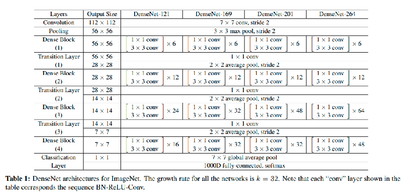
As we can see, the network starts with a convolution layer followed by a polling layer, we will call this the “start” layer, the we will add the Dense Blocks with repetitions of 6, 12, 24 and 16 times (with transition layers between them), then we will add a global average pooling (AggregationLayer) and a 1000 neuron fully connected softmax layer, we will call this “Tail Layer”.
In[]:=
network=NetChain[{(**Startlayer**)ConvolutionLayer[64,7,"Stride"2,"PaddingSize"{3,3}],PoolingLayer[3,2,"PaddingSize"{1,1},"Function"Max],(**Denseblocks**)DenseBlock[6,32],TransitionLayer[256],DenseBlock[12,32],TransitionLayer[512],DenseBlock[24,32],TransitionLayer[1024],DenseBlock[16,32],(**Taillayer**)AggregationLayer[Mean],LinearLayer[1000],SoftmaxLayer[]},"Input"NetEncoder[{"Image",{224,224}}]]
Out[]=
NetChain
 | uniniti alized |
|
Usability
Usability
We will now apply the architecture we have created for DenseNet-121 over the Flowers dataset, which contains 4242 images of flowers divided into five classes: daisy, tulip, rose, sunflower, dandelion. For each class there are about 800 photos with resolution of about 320x240 pixels.
Data loading
Data loading
We have downloaded the dataset from the source and once we have it in our computer we load it from the directory, the data folder has subfolders for each flower class containing the corresponding images. We will create an association map with the images paths as keys and the image classes as values. Because this example is only for showing the usability of the network, we will take only 2 classes of flowers, this will reduce the training time.
Data directory
In[]:=
dir="C:\\Users\\ECF0124A\\Downloads\\flowers";
Create loadFiles function that creates association map between image files and class
In[]:=
loadFiles[dir_]:=Map[File[#]FileNameTake[#,{-2}]&,FileNames["*.jpg",dir,Infinity]];
Data set association map creation
In[]:=
data=loadFiles[dir];
Rose and sunflower class selection
In[]:=
data2=Select[data,Values[#]"rose"||Values[#]"sunflower"&];
Data exploration
Data exploration
Having a look over the dataset, allows to evaluate the quality of the data and see if the data has the content type expected.
Image collage of flowers dataset
In[]:=
ImageCollage[Map[Import,Join[RandomSample[FileNames["*.jpg",FileNameJoin[{dir,"sunflower"}]],2],RandomSample[FileNames["*.jpg",FileNameJoin[{dir,"rose"}]],2]]]]
Out[]=

Data distribution of classes
In[]:=
BarChartCounts[Values[data2]],
Out[]=

We can also observe the distribution of image classes is almost balanced, so it wont be a problem for the training process.
Data splitting into train and test sets
Data splitting into train and test sets
Before training, we need to split the data into train and test sets, this allows to make an evaluation of the model performance after training.
Call TrainTestSplit function from the Resource Function Repository
In[]:=
split=ResourceFunction["TrainTestSplit"];
Split the dataset into train and test sets in a 80/20 proportion
In[]:=
splitData=split[data2,"TestSetSize"Scaled[0.1]];
Define test and train sets separately
In[]:=
train=splitData[[1]];test=splitData[[2]];
Data distribution of classes in train and test sets
In[]:=
BarChart{Counts[Values[train]],Counts[Values[test]]},
Out[]=

Creating custom DenseNet-121
Creating custom DenseNet-121
Before training, we need to modify the DenseNet we have created, we need to adapt the last 2 layers to the specific task we are working on, making the output have 5 neurons instead of 1000.
Remove the last 2 layers from the previously constructed DenseNet-121, this allows to customize the network with the amount of desired output classes
In[]:=
customNetwork=Take[network,{1,-3}]
Out[]=
NetChain
| uniniti alized |
|
Crate a custom Neural Network including 5 output classes to the DenseNet-121, we added ImageAugmentationLayer that applies random image transformations over the training set
In[]:=
newNet=NetChain[<|"Augm"ImageAugmentationLayer[{224,224},"Input"NetEncoder[{"Image",{300,300}}]],"densenet"customNetwork,"linear"LinearLayer[2],"softmax"SoftmaxLayer[]|>,"Output"NetDecoder[{"Class",{"sunflower","rose"}}]]
Out[]=
NetChain
| uniniti alized |
|
Model training
Model training
Model training over the train data set with 1 round and LearningRate=0.00001
In[]:=
trainedNet=NetTrain[newNet,train,MaxTrainingRounds1,BatchSize8,LearningRate0.00001]
Out[]=
NetChain
|
|
Model evaluation
Model evaluation
Accuracy
In[]:=
NetMeasurements[trainedNet,test,"Accuracy"]
Out[]=
0.907895
Confusion Matrix
In[]:=
NetMeasurements[trainedNet,test,"ConfusionMatrixPlot"]
Out[]=
actual class |  |
| predicted class |
In[]:=
NetMeasurements[trainedNet,test,"ConfusionMatrixPlot"]
ROC Curve
In[]:=
NetMeasurements[trainedNet,test,"ROCCurvePlot"]
Out[]=
recall |  |
| false positive rate |
Concluding comments
Concluding comments
We have constructed a Densely Connected Convolutional Network named DenseNet-121 from scratch and described its basic constructing blocks. The code we have written can be also be modified to fit the architecture of the other known denseNets (DenseNet-169, DenseNet-201 and DenseNet-264). The architecture was not trained on any dataset as for example ImageNet, nevertheless it can be useful for image classification taking into account it wont be transfer learning. We have tested the architecture usability training over a flower classification dataset, obtaining 90% of accuracy.
Acknowledgment
Acknowledgment
I’d like to thank Tuseeta Banerjee (WRI) for her valuable technical help, and Mads Bahrami (WRI) for his suggestions and reviews helping to improve this essay.
References
References
Cite this as: siria Sadeddin, "Densely Connected Convolutional Networks: construction and application" from the Notebook Archive (2021), https://notebookarchive.org/2021-01-8cj1uw9
Download
