Deriving Formulas for Pretty 3D Polygons
Author
Tom Verhoeff
Title
Deriving Formulas for Pretty 3D Polygons
Description
This notebook demonstrates how to derive formulas and find exact solutions for some of the pretty 3D polygons designed by Koos Verhoeff in the 1990s.
Category
Academic Articles & Supplements
Keywords
3D polygons, turtle geometry, symmetry
URL
http://www.notebookarchive.org/2021-08-7dhhwzg/
DOI
https://notebookarchive.org/2021-08-7dhhwzg
Date Added
2021-08-16
Date Last Modified
2021-08-16
File Size
379.02 kilobytes
Supplements
Rights
CC BY-NC-SA 4.0

Deriving Formulas for Pretty 3D Polygons
Deriving Formulas for Pretty 3D Polygons
Eindhoven University of Technology, Netherlands
This notebook demonstrates how to derive formulas and find exact solutions for some of the pretty 3D polygons designed by Koos Verhoeff in the 1990s. It serves as supplementary material for the article “Pretty 3D Polygons: Explorations and Proofs” by Melissa van Veenendaal and Tom Verhoeff, which was
presented at the Bridges Conference about Mathematics & Arts in 2021.
presented at the Bridges Conference about Mathematics & Arts in 2021.
In[]:=
Preliminaries
Preliminaries
To study 3D paths in space, such as that wonderful star shape shown above, it can be helpful to describe the path not extrinsically through points with (ugly) coordinates, but rather intrinsically as the product of a (flying or swimming) turtle that moves in 3D space according to a (simple) program.
The 3D turtle can be instructed to trace out a path in space by giving it a sequence of turtle commands. The semantics of these turtle commands is defined in terms of how they operate on the turtle’s state, which consists of three vectors: position, heading, and normal. In the initial state, the turtle is positioned in the origin, heading in the direction of the positive x-axis, with its normal vector pointing in the direction of the z-axis. The Wolfram Demonstrations Project “3D Flying Pipe-Laying Turtle” lets you experiment with such a turtle and see the paths that it constructs. Here we are interested in analyzing such turtle programs, rather than drawing pictures.
In[]:=
(*initialstate*)istate={{0,0,0},{1,0,0},{0,0,1}};(*indicestoextractpartsofastate*){pos,hdg,nrm}={1,2,3};
In[]:=
istate[[{pos,hdg,nrm}]]
Out[]=
{{0,0,0},{1,0,0},{0,0,1}}
The three basic commands in a turtle program are defined as parameterized state transformers:
In[]:=
(*movetheturtleforwardalongitsheadingvectorbydistanced*)move[d_][{position_,heading_,normal_}]:={position+dheading,heading,normal}(*turntheturtleaboutitsnormalvectorbyanglephi*)turn[phi_][{position_,heading_,normal_}]:={position,Cos[phi]heading+Sin[phi]Cross[normal,heading],normal}(*rolltheturtleaboutitsheadingvectorbyanglepsi*)roll[psi_][{position_,heading_,normal_}]:={position,heading,Cos[psi]normal-Sin[psi]Cross[normal,heading]}
Commands can be composed into programs by sequencing. The semantics of such a composition is given by the following state transformer.
In[]:=
seq[][state_]:=stateseq[cmd_,rest___][state_]:=seq[rest][cmd[state]]
If you wish, nested uses of seq can be eliminated:
In[]:=
simplify[seq[t___,seq[u___],v___]]:=simplify[seq[t,u,v]]simplify[arg_]:=arg
All turtle paths can be expressed as a suitable composition of the following program fragment with just three parameters, a move distance, a turn angle, and a roll angle (but note that the turtle rolls before it turns):
In[]:=
segment[d_,psi_,phi_]:=seq[move[d],roll[psi],turn[phi]]
To achieve rotation symmetry, a program fragment can be repeated:
In[]:=
repeat[prog_,n_]:=seq@@Table[prog,n]
Pretty 3D polylines have a fixed move distance d, a fixed turn angle phi (the angle between adjacent segments then equals 180º minus phi), and a fixed roll angle psi whose signs are taken from the string s through the following function:
In[]:=
prettypoly[s_,d_,psi_,phi_]:=seq@@Table[segment[d,factor[c]psi,phi],{c,Characters[s]}](*convertasigncharacterintoamultiplicativefactor*)factor[c_]:=Switch[c,"+",+1,"-",-1]
A pretty 3D polygon is a pretty 3D polyline that closes properly, that is, it returns to the initial state.
Koos’ Star Problem
Koos’ Star Problem
Koos considered the following pretty 3D polyline, which is a function of turn angle phi:
In[]:=
repeat[prettypoly["++--",1,90°,phi],4]//simplify
Out[]=
seq[move[1],roll[90°],turn[phi],move[1],roll[90°],turn[phi],move[1],roll[-90°],turn[phi],move[1],roll[-90°],turn[phi],move[1],roll[90°],turn[phi],move[1],roll[90°],turn[phi],move[1],roll[-90°],turn[phi],move[1],roll[-90°],turn[phi],move[1],roll[90°],turn[phi],move[1],roll[90°],turn[phi],move[1],roll[-90°],turn[phi],move[1],roll[-90°],turn[phi],move[1],roll[90°],turn[phi],move[1],roll[90°],turn[phi],move[1],roll[-90°],turn[phi],move[1],roll[-90°],turn[phi]]
All the edges have the same (unit) length, all the angles between adjacent edges are equal (to 180º minus phi degrees), and all roll angles are +90º or -90º according to the given string with signs. So, it consists of 16 edges. Koos faced the following problem: do there exist turn angles phi for which this program produces a nicely closed path, that is, where the turtle returns to its initial state? Note that in order for the first and the last edge to make that same angle phi (and also for the roll to work out nicely), the turtle in fact needs to return to its initial heading and normal. When such a turn angle phi exists, the result is a pretty 3D polygon with nice rotation and reflection symmetries (see the figure above). The following image shows a choice of phi which does not close.
Koos worked out his designs based on numerical approximations of conjectured solutions. The accompanying article shows that such solutions indeed exist, and this notebook shows how to derive formulas for analytic solutions.
Pretty 3D polygon based on (+−)^3
Pretty 3D polygon based on (+−)^3
We start with a simpler pretty 3D polygon.
In[]:=
prp3=repeat[prettypoly["+-",1,Pi/2,phi°],3]//simplify
Out[]=
seqmove[1],roll,turn[°phi],move[1],roll-,turn[°phi],move[1],roll,turn[°phi],move[1],roll-,turn[°phi],move[1],roll,turn[°phi],move[1],roll-,turn[°phi]
π
2
π
2
π
2
π
2
π
2
π
2
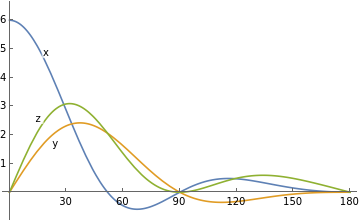
The final position as function of the turn angle phi for (+−)^3:
In[]:=
prp3[istate][[pos]]//TrigReduce
Out[]=
(16+26Cos[°phi]+24Cos[2°phi]+21Cos[3°phi]+8Cos[4°phi]+Cos[5°phi]),(6Sin[°phi]+10Sin[2°phi]+6Sin[3°phi]+Sin[4°phi]),(18Sin[°phi]+16Sin[2°phi]+19Sin[3°phi]+8Sin[4°phi]+Sin[5°phi])
1
16
1
8
1
16
This needs to equal istate[[pos]] to have closure. For proper closure, also the final heading and final normal need to equal the initial heading and normal. Here is the full set of nine equations to solve for proper closure in the approach before the technique in the article was developed:
In[]:=
istate==prp3[istate]//TrigReduce
Out[]=
{{0,0,0},{1,0,0},{0,0,1}}(16+26Cos[°phi]+24Cos[2°phi]+21Cos[3°phi]+8Cos[4°phi]+Cos[5°phi]),(6Sin[°phi]+10Sin[2°phi]+6Sin[3°phi]+Sin[4°phi]),(18Sin[°phi]+16Sin[2°phi]+19Sin[3°phi]+8Sin[4°phi]+Sin[5°phi]),(14-16Cos[°phi]-Cos[2°phi]+8Cos[3°phi]+18Cos[4°phi]+8Cos[5°phi]+Cos[6°phi]),(6Sin[°phi]-4Sin[2°phi]+7Sin[3°phi]+6Sin[4°phi]+Sin[5°phi]),(-8Sin[°phi]-3Sin[2°phi]+16Sin[4°phi]+8Sin[5°phi]+Sin[6°phi]),(-6Sin[°phi]+4Sin[2°phi]-7Sin[3°phi]-6Sin[4°phi]-Sin[5°phi]),(-1-4Cos[°phi]+4Cos[3°phi]+Cos[4°phi]),(2+10Cos[°phi]-8Cos[2°phi]+5Cos[3°phi]+6Cos[4°phi]+Cos[5°phi])
1
16
1
8
1
16
1
32
1
16
1
32
1
16
1
8
1
16
Mathematica can in fact solve this:
In[]:=
Solve[istate==prp3[istate]//TrigReduce,phi,Reals]//Simplify
Out[]=
phi if ∈,phi if ∈
π(-1+4)
1
2°
1
π+4π
1
2°
1
Thus, phi = π/2. This pretty polygon turns out to be a path on the cube, avoiding two diametrically opposite vertices. Note that the following cell contains a 3D graphics object that can be manipulated.
In[]:=
Final position plotted as function of turn angle phi (target is {0, 0, 0}):
In[]:=
Plot(16+26Cos[°phi]+24Cos[2°phi]+21Cos[3°phi]+8Cos[4°phi]+Cos[5°phi]),(6Sin[°phi]+10Sin[2°phi]+6Sin[3°phi]+Sin[4°phi]),(18Sin[°phi]+16Sin[2°phi]+19Sin[3°phi]+8Sin[4°phi]+Sin[5°phi]),{phi,0,180},PlotLabelsPlaced[{"x","y","z"},{{15,Above},{20,Below},{20,Above}}],Ticks{{30,60,90,120,150,180},{1,2,3,4,5,6}}
1
16
1
8
1
16
Out[]=

Final heading plotted as function of phi (target is {1, 0, 0}):
In[]:=
Plot(14-16Cos[°phi]-Cos[2°phi]+8Cos[3°phi]+18Cos[4°phi]+8Cos[5°phi]+Cos[6°phi]),(6Sin[°phi]-4Sin[2°phi]+7Sin[3°phi]+6Sin[4°phi]+Sin[5°phi]),(-8Sin[°phi]-3Sin[2°phi]+16Sin[4°phi]+8Sin[5°phi]+Sin[6°phi]),{phi,0,180},PlotLabelsPlaced[{"x","y","z"},{{5,Above},{30,Above},{30,Above}}],Ticks{{30,60,90,120,150,180},Automatic}
1
32
1
16
1
32
Out[]=

Final normal plotted as function of phi (target is {0, 0, 1}):
In[]:=
Plot(-6Sin[°phi]+4Sin[2°phi]-7Sin[3°phi]-6Sin[4°phi]-Sin[5°phi]),(-1-4Cos[°phi]+4Cos[3°phi]+Cos[4°phi]),(2+10Cos[°phi]-8Cos[2°phi]+5Cos[3°phi]+6Cos[4°phi]+Cos[5°phi]),{phi,0,180},PlotLabelsPlaced[{"x","y","z"},{{20,Below},{20,Above},{20,Above}}],Ticks{{30,60,90,120,150,180},Automatic}
1
16
1
8
1
16
Out[]=

The difficulty with this approach is that one needs to solve a system of nine equations, and although each equation clearly has solutions, it is not clear why they would have simultaneous solutions.
Koos’ Star based on (++−−)^4
Koos’ Star based on (++−−)^4
The 3D turtle program underlying Koos’ Star:
In[]:=
KS[phi_]:=repeat[prettypoly["++--",1,π/2,phi],4]
In[]:=
KS[phi]//simplify
Out[]=
seqmove[1],roll,turn[phi],move[1],roll,turn[phi],move[1],roll-,turn[phi],move[1],roll-,turn[phi],move[1],roll,turn[phi],move[1],roll,turn[phi],move[1],roll-,turn[phi],move[1],roll-,turn[phi],move[1],roll,turn[phi],move[1],roll,turn[phi],move[1],roll-,turn[phi],move[1],roll-,turn[phi],move[1],roll,turn[phi],move[1],roll,turn[phi],move[1],roll-,turn[phi],move[1],roll-,turn[phi]
π
2
π
2
π
2
π
2
π
2
π
2
π
2
π
2
π
2
π
2
π
2
π
2
π
2
π
2
π
2
π
2
The following would take very long to evaluate (that is why it is commented out):
In[]:=
(*KS[phi][istate][[pos]]//TrigReduce*)
So, a direct solution is out of reach. The accompanying article explains how to exploit the symmetries.
A turtle program can be reflected in the plane perpendicular to its final heading vector, by reversing the commands and flipping the signs of all roll commands:
In[]:=
reflfh[move[d_]]:=move[d]reflfh[roll[psi_]]:=roll[-psi]reflfh[turn[phi_]]:=turn[phi]reflfh[seq[seq___]]:=seq@@Table[reflfh[cmd],{cmd,Reverse[{seq}]}]
By cyclically shifting half of the last turn command to the front, we can rewrite KS[phi] as (P[phi]; reflfh[P[phi]])^4, where P is defined by
In[]:=
P[phi_]:=seq[turn[phi/2],move[1],roll[Pi/2],turn[phi],move[1],roll[Pi/2],turn[phi/2]]
In[]:=
seq[P[phi],reflfh[P[phi]]]//simplify

phi
2
π
2
π
2
phi
2
phi
2
π
2
π
2
phi
2
phi
2
π
2
π
2
phi
2
Out[]=
seqturn,move[1],roll,turn[phi],move[1],roll,turn,Applyturn,move[1],roll,turn[phi],move[1],roll,turn,turn,roll-,move[1],turn[phi],roll-,move[1],turn
phi
2
π
2
π
2
phi
2
phi
2
π
2
π
2
phi
2
phi
2
π
2
π
2
phi
2
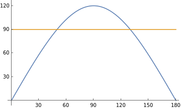
The rotation angle theta between initial and final heading of the repeated part (P[phi]; reflfh[P[phi]]) is twice the angle between the reflection planes which have as normal vectors istate[[hdg]] and P[phi][istate][hdg]. The dot product between these normal vectors gives us the cosine of half the rotation angle:
In[]:=
thetaKS[phi_]:=2ArcCos[Dot[istate[[hdg]],P[phi][istate][[hdg]]]//TrigReduce]
In[]:=
thetaKS[phi]
Out[]=
2ArcCos(3+Cos[2phi])
1
4
In[]:=
Plot[{thetaKS[phi°]/°,90},{phi,0,180},Ticks{{30,60,90,120,150,180},{30,60,90,120,150,180}}]
Out[]=

To get a properly closed pretty 3D polygon from 4 repetitions, the rotation angle should equal 90º:
In[]:=
Solve[thetaKS[phi]Pi/2,phi,Reals]
Out[]=
phi-ArcCos[-3+2 if ∈,phiArcCos[-3+2 if ∈
1
2
2
]+2π
1
1
1
2
2
]+2π
1
1
In[]:=
NSolve[thetaKS[phi°]Pi/2,phi,Reals]//Simplify
Out[]=
phi,phi
-49.9396+180. if ∈
1
1
49.9396+180. if ∈
1
1
In[]:=
The angle between adjacent segments for the other solution (shown below):
In[]:=
180-49.939640973639314`
Out[]=
130.06
In[]:=
Proper Closure of Other Pretty Polygons: Generalizations
Proper Closure of Other Pretty Polygons: Generalizations
To exploit the reflection symmetry in general, let us shift all segments cyclically over phi/2:
In[]:=
segment2[d_,psi_,phi_]:=seq[turn[phi/2],move[d],roll[psi],turn[phi/2]]prettypoly2[s_,d_,psi_,phi_]:=seq@@Table[segment2[d,factor[c]psi,phi],{c,Characters[s]}]theta[prog_][phi_]:=2ArcCos[Dot[istate[[hdg]],prog[phi][istate][[hdg]]]//TrigReduce]
Pretty 3D polygon based on (+++−−−)^4
Pretty 3D polygon based on (+++−−−)^4
In[]:=
P3[phi_]:=prettypoly2["+++",1,Pi/2,phi]theta3:=theta[P3]
In[]:=
P3[phi]//simplify
Out[]=
seqturn,move[1],roll,turn,turn,move[1],roll,turn,turn,move[1],roll,turn
phi
2
π
2
phi
2
phi
2
π
2
phi
2
phi
2
π
2
phi
2
In[]:=
theta3[phi]
Out[]=
2ArcCos(6+3Cos[phi]-2Cos[2phi]+Cos[3phi])
1
8
In[]:=
Plot[{theta3[phi°]/°,90},{phi,0,180},Ticks{{30,60,90,120,150,180},{30,60,90,120,150,180}}]
Out[]=

In[]:=
NSolve[theta3[phi°]Pi/2,phi,Reals]//Simplify
Out[]=
phi,phi
-127.176+360. if ∈
1
1
127.176+360. if ∈
1
1
The angle between adjacent segments of design shown below:
In[]:=
180-127.17632078275625`
Out[]=
52.8237
In[]:=
Pretty 3D polygon based on (++−++−−+−−)^3
Pretty 3D polygon based on (++−++−−+−−)^3
In[]:=
P5[phi_]:=prettypoly2["++-++",1,Pi/2,phi]theta5:=theta[P5]
In[]:=
P5[phi]//simplify
Out[]=
seqturn,move[1],roll,turn,turn,move[1],roll,turn,turn,move[1],roll-,turn,turn,move[1],roll,turn,turn,move[1],roll,turn
phi
2
π
2
phi
2
phi
2
π
2
phi
2
phi
2
π
2
phi
2
phi
2
π
2
phi
2
phi
2
π
2
phi
2
In[]:=
theta5[phi]
Out[]=
2ArcCos(14+6Cos[phi]+9Cos[3phi]+2Cos[4phi]+Cos[5phi])
1
32
In[]:=
Plot[{theta5[phi°]/°,120},{phi,0,180},PlotRangeAll,Ticks{{30,60,90,120,150,180},{30,60,90,120,150,180}}]
Out[]=

In[]:=
NSolve[theta5[phi°]2Pi/3,phi,Reals]//Simplify
Out[]=
phi,phi,phi,phi,phi,phi
-90.+360. if ∈
1
1
90.+360. if ∈
1
1
-31.9646+360. if ∈
1
1
31.9646+360. if ∈
1
1
-131.376+360. if ∈
1
1
131.376+360. if ∈
1
1
The angle between adjacent segments of the design shown below:
In[]:=
180-131.37561290976313`
Out[]=
48.6244
In[]:=
The other two solutions:
(End of Notebook)
Cite this as: Tom Verhoeff, "Deriving Formulas for Pretty 3D Polygons" from the Notebook Archive (2021), https://notebookarchive.org/2021-08-7dhhwzg
Download
