Computational Essay, Data Visualization, Astronomy, Earth Science, Meteorites, Data Analytics
URL
http://www.notebookarchive.org/2020-12-47jpn80/
DOI
https://notebookarchive.org/2020-12-47jpn80
Date Added
2020-12-09
Date Last Modified
2020-12-09
File Size
20.21 megabytes
Supplements
Rights
Redistribution rights reserved
Download
Open in Wolfram Cloud
Exploring meteorite landing data
Laney Moy
In this essay, I explore different properties of meteorite landing records in order to identify changes and patterns in the tracking of meteorite landings over time and location. The data cover landing records across the globe from the 14th century until 2013 and contain information about mass, classification, location, and more. The landing records are available through the Wolfram Data Repository or NASA's Open Data Portal, and both import methods are compatible with the analysis below.
has meteorite landing data for 45,716 landings, which are included in the downloadable CSV file on the site. I imported the file and iconized the resulting raw data, which we can format properly for the rest of the essay.
Use iconized raw data from the CSV file:
In[]:=
meteoriteData=
MeteoritedatafromNASAOpenDataPortalCSV
;
Create functions to parse Strings into appropriate objects and remove missing objects:
What’s actually contained in these records? Let’s take a look.
Here’s the data for an arbitrary meteorite landing.
Retrieve data for a meteorite landing:
In[]:=
meteoriteData[73]
Out[]=
The name and ID are pretty self-explanatory and serve as identification for the meteorite landing.
The next heading is NameType, for which the options are “Valid” and “Invalid.” Valid meteorites still had meteoritical composition upon discovery after landing, whereas invalid meteorites had decomposed until their composition no longer had typical meteoritical properties. The vast majority of meteorites in this dataset are valid.
Count the number of each NameType:
In[]:=
meteoriteData[Counts,"NameType"]
Out[]=
The class, under the heading “Classification,” of a meteorite designates its composition class. Some common classes are the L and H categories. There are 455 different classifications.
Count the number of Classification categories:
In[]:=
meteoriteData[CountDistinct,"Classification"]
Out[]=
455
The mass of each meteorite is listed in grams.
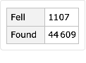
The heading “Fall” corresponds to whether a meteorite landing was noticed on its way to Earth and recorded immediately after falling (“Fell”) or discovered after the fact, usually much later (“Found”).
Count the number of each Fall category:
In[]:=
meteoriteData[Counts,"Fall"]
Out[]=
The year corresponds to the date on which the landing was recorded. All dates are listed as midnight on the first of the year in which they landed.
“Coordinates” indicates the location of a landing. “Found” meteorites have no location data because the meteorite remains may have moved between landing and discovery.
Create a GeoHistogram of the locations of all meteorite landings:
As an initial exploration, we can take a look at the masses of the meteorites in this collection. We’ll use what we discover to inform the rest of the investigation. Let’s first try running all of the mass data through a histogram.
Most of these meteorites are quite small! The leftmost bar contains significantly more meteorites than any other bar, and the data set is skewed to the right.
Let’s calculate some statistics about this distribution.
The median is 32.6 grams while the mean is 13,278.1 grams. The spread of the minimum, quartiles, and maximum is also quite interesting -- the first and second quartile are fairly close while the third quartile and maximum are significantly higher. These statistics verify what we noticed earlier -- the data are very right-skewed!
What type of distribution might best represent our data?
Interesting, a mixture of a LogNormalDistribution and a UniformDistribution. Since it’s mostly a LogNormalDistribution, it rises suddenly at the beginning and then curves sharply downward as the mass increases to the right. As expected, the distribution is quite skewed to the right.
We’ve discovered that there’s an enormous number of small meteorites with some quite massive larger meteorites.
Filtering data
In order to explore some differences between these groups moving forward, I make a smaller dataset here only with large meteorites. Working with a smaller dataset is also useful for more computationally intensive tasks later.
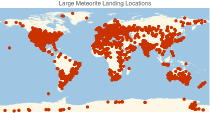
Select landings by meteorites with a mass greater than or equal to 1,000 grams:
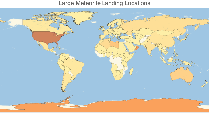
We can see red clusters in certain areas of the map, particularly in North America and Europe. We can take a look at meteorite landings by country as well.
Neat! The United States has a pretty high number of meteorite landings recorded, which makes sense based on its geographical size and interest in collecting astronomical data. Interestingly, Antarctica has a high number of recorded landings as well. According to NASA’s Meteors and Meteorites page, meteorites are more often found and identified in deserts, including Antarctica, where they are more easily distinguishable from the surrounding environment.
Let’s create some GeoHistograms not separated by country to see where hotspots are globally.
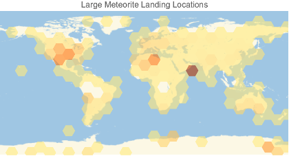
Make a GeoHistogram based on the locations of large meteorite landings:
There are some hotspots in the central United States, at some locations along the Mediterranean coast and in Europe, and on the edge of the Arabian peninsula.
Now, I make another GeoHistogram -- this time including smaller meteorite landings as well.
Make a GeoHistogram based on the locations of all meteorite landings:
Whoa! While there are still some orange areas in the Arabian peninsula, North Africa, and the United States, some of the darkest areas are in Antarctica.
That means that a large number of smaller meteorites have been found in the Antarctic desert.
Let’s take a look at how the geographic distribution of large meteorite landing records changed over time. I’ll use the Animate function to create a simple visualization. This is pretty computationally intensive, so we’ll use the large meteorites only.
I don’t want to have to recalculate which locations are necessary in every frame, so I’ll make a Table of locations first.
Make a List of large meteorite landing locations for each 20-year period between 1700 and 2020:
Animate the locations of recorded large meteorite landings in each 20-year period between 1700 and 2020:
In[]:=
ListAnimate[geoListPlots,AnimationRate1]
Out[]=
Large meteorite landing records seem to be concentrated in North America, Europe, and Antarctica and have increased over the years.
Let’s take a closer look at temporal patterns in meteorite records.
Meteorite landing records over time
Let’s take a look at a DateHistogram of the records for the largest meteorites.
I’d like to separate meteorites categorized as “Fell” and those categorized as “Found” because “Found” meteorites were discovered after the actual date when they landed.
Group the large meteorite landing data by “Fell” and “Found” categorization:
The “Fell” dataset is much smaller than the “Found” dataset with only 282 landings compared to 1106 landings. That means that most large meteorites are found after they reach Earth. We’ll take a closer look at this later in the essay. For now, onward!
Now that I’ve selected only those meteorites, let’s make histograms.
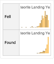
Make DateHistograms from the years of large meteorite landings:
Interesting! Let's take a look at them together as well. We use a log scale because otherwise the later counts for “Found” meteorites grows so much that the rest of the plot is barely visible.
Make a DateHistogram of the “Fell” and “Found” meteorite landing years:
As we noticed earlier, the “Found” meteorite landings outnumber the “Fell” meteorite landings. Records of “Fell” meteorite landings appear to have increased until around 1860 and since remained fairly stable, while “Found” meteorite landings have continued increasing by quite a lot. This makes sense -- while a limited number of meteorites land on Earth each year, technology and an interest in research has likely allowed for a higher number of old meteorites to be found in recent decades.
What about landings of meteorites less than 1,000 grams? Let’s separate the “Fell” and “Found” categories again.
Group the meteorite landing data by “Fell” and “Found” categorization:
In[]:=
allMeteoritesFall=meteoriteData[GroupBy["Fall"]];
Get the number of “Fell” and “Found” meteorites:
In[]:=
allMeteoritesFall[All,Length]
Out[]=
Great! Again, the “Found” meteorite landings far outnumber the “Fell” landings.
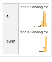
Make DateHistograms from the years of large meteorite landings:
When we take into account smaller meteorites, the “Found” meteorite landings outnumber the “Fell” landings to an even greater degree, especially in the past century. This indicates that in recent years there has been fairly significant discovery of smaller meteorites that had previously gone unnoticed.
Let’s take a look at the differences between the large meteorite statistics and all meteorite statistics.
Make a DateHistogram comparing the landing years of large meteorites and all meteorites in the category “Fell”:
The shape of the overlaid histograms looks pretty similar, so smaller meteorite landings that are recorded at the time of falling are being tracked similarly regardless of size.
Make a DateHistogram comparing the landing years of large meteorites and all meteorites in the category “Found”:
Based on this histogram, which is overwhelming blue and having much increased over the years, smaller meteorite landings have been discovered and recorded at an extremely high rate relative to large meteorite landings.
Since we’ve looked a lot at large meteorites compared to small meteorites, we can also look at a scatterplot showing the relationship between mass and year.
Make a scatterplot of the years and masses of all meteorite landing records:
Overall, the distribution looks fairly random at first and later becomes more densely packed, especially among smaller “Found” meteorites in more recent years. This is consistent with the earlier histograms.
We’ve discovered that humans have found a lot of meteorites, especially small meteorites, in recent years!
Classifications
Let’s take a look at the type classifications of large meteorites that have landed on Earth. What kinds of meteorites are most frequently found and recorded?
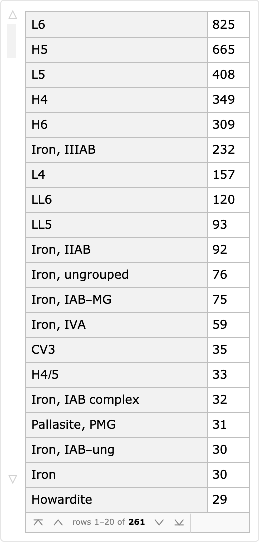
Calculate the number of large meteorites in each class:
I put the information in a bar graph. Since there are many classes, their labels would overlap quite a bit, so hover over each bar to see its classification.
The most frequent large meteorite classifications are H type, L type, and iron. H and L type chrondites are the very common meteorite classifications, so it makes sense that they make up many of these meteorites. Although iron meteorites do not actually make up a high percentage of meteorites, they are consistently overrepresented in meteorite landing data because they are easily recognizable and resistant to weathering and decay.
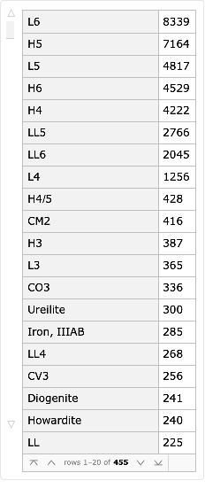
Let’s make another bar chart of the most common classifications for all meteorite landings.
In this bar chart, all of the most common types are H and L chrondites. This makes sense because these two classifications are so common, and likely large iron meteorites do not skew the data as much as in the last bar chart.
Most meteorites that have been found on earth are L chrondites, along with H chrondites. The most common category is L6. Let’s take a look at where L6 chrondites are found.
Make a GeoHistogram of the locations of L6 meteorite landings:
Most of these have been found in the Antarctic. Since L6 meteorites are usually small and lighter colored, it seems reasonable that they are frequently found in the frozen desert.
Overall, people seem to have mostly found L and H chrondites, along with many large iron meteorites.
Conclusion
By exploring meteorite landing data, we’ve discovered the following:
◼
The vast majority of meteorites that have been recorded as landing on Earth are small.
◼
Meteorites are most frequently found in North America, the tip of the Arabian peninsula, North Africa, and Antarctica. Most of these locations have topography compatible with identifying meteorites.
◼
Over time, people have been finding more meteorites, especially small ones that landed in the past. The number of landing records in recent years have skyrocketed.
◼
Most of the meteorites found are H and L chrondites, which are small and most often found in deserts, where they are most easily visible, but also all over the world.
Through investigating meteorite landings, we found a number of patterns in how people track and record meteorites.