Holistic Mathematics, vol. 2
Author
John Erickson
Title
Holistic Mathematics, vol. 2
Description
We use a recreational discrete math problem to explore issues in math and math education.
Category
Educational Materials
Keywords
math, recreational math, discrete math, math education
URL
http://www.notebookarchive.org/2021-02-5k5j0pk/
DOI
https://notebookarchive.org/2021-02-5k5j0pk
Date Added
2021-02-12
Date Last Modified
2021-02-12
File Size
2.77 megabytes
Supplements
Rights
CC BY-NC-SA 4.0

Holistic Mathematics: Experiments, Computation, and Proof: Vol 2
Holistic Mathematics: Experiments, Computation, and Proof: Vol 2
John Erickson, PhD
“I don’t want to belong to any club that would have me as a member.” -Groucho Marx
“A recent (published) paper had near the beginning the passage `The object of this paper is to prove (something very important).’ It transpired with great difficulty, and not till near the end, that the `object’ was an unachieved one.” -Littlewood’s Miscellany

Prologue to all 4 volumes (abridged)
Prologue to all 4 volumes (abridged)
This monograph is a bit weird, but maybe it’s time for a little weird because normal and conventional has clearly not worked out so well when it comes to some of the problems in math education in my opinion.
There are several goals for this four volume monograph. Too many times students have asked me “How do you do research in mathematics?” and I have found that the best way, perhaps the only way, is to just do some research with them. Since that isn’t a scalable solution, my main goal is to illustrate, at a fairly elementary level, one approach to how math research can be done by providing a concrete and comprehensive, albeit vicarious, research experience which goes “from grammar school to graduate school”. I put that in quotes because I thought I made it up, but I’m apparently not the only one who says this. In order to facilitate this goal, I have sort of “let it all hang out” so to speak, nothing gross mind you, I just haven’t removed all the evidence of work, false approaches, incorrect ideas, and shortcomings. This gives the monograph a rough quality, but that is not intended as an excuse for actual mistakes, of which I am sure there are many.
The problem which started our investigation was an essentially randomly chosen elementary recreational discrete math problem. Someone sent me their kids math circle problem. Now, I make no claim to being a great mathematician and, in particular, I am not really all that great at discrete mathematics. Contrary to this being a deficit however, this was actually an advantage for my goals, since an expert would likely know the standard machinery and be done with it. I, on the hand, actually had to think about the problem and create some code to make sure I understood what was going on. After solving the problem I decided I would see what would happen if I just followed the mathematics to see where it led through the standard process of both generalization and specialization. In the end, I would say that the journey wound up being a seemingly random “stop and smell the roses” tour of mathematics. Speaking of the “end”, my stopping criteria, that I end up at the graduate level, was a bit problematic since it took about three years and perhaps I only ended up at the advanced undergraduate beginning graduate student level. If you’re the sort that likes to know where you are going before you begin a journey, the last result, in volume 4, is from computational and theoretical combinatorial group theory. Alexander Hulpke and I added sequence A337015 to the OEIS and proved a nice but simple theorem connecting sequences A005432 and A337015 which makes one ask how else these sequences might be related. One question I find interesting to ask is the following: if I started with the exact same problem today would I end up three years later arriving at the same terminal result or not?
Just to be absolutely clear, there is really nothing original in my approach, which is probably most influenced by Polya, Ross, and even Moore (sans all of his racism) along with various teachers and professors I have had. I would say that it is also heavily influenced by my modest knowledge of experimental mathematics and the use of software to do calculations. I used Mathematica primarily along with the OEIS, but I also used WolframAlpha, the Inverse Symbolic Calculator, and GAP as well. There are many choices for tools and the underlying mathematics does not depend on those choices. Here is an interesting related issue regarding the balance of math and computation. I have noticed that a lot of students who like coding neglect math these days, and would be quite happy if they never saw another equation again. I find this situation unfortunate. On the other hand, I have also been told by well meaning, and very smart math people, that I should remove or otherwise segregate all the code in these volumes. I said to myself, “Yeah, that ain’t ever gonna happen.” Am I in love with my own code and just being stubborn you ask? I don’t think so. Obviously, I think learning to code is important, but the primary reason I have left the code in place is that I am firmly convinced that the tendency to present the slick final product of our mathematical labors in the form of an elegant proof without the motivations, experiments, and even incorrect understandings, is part of the reason so many students turn away from mathematics. They say to themselves, “Well, I could never do that, I better switch majors.” This is particularly true for students who are already insecure, in particular, members of underrepresented groups.
The basic process we will follow throughout the volumes is simple, and is what mathematicians do all the time: play with some mathematical problem, consider examples, run experiments, look at visualizations, notice patterns, make conjectures and try to prove them. Inevitably, you will make new definitions and generalizations and find new patterns, make new conjectures, prove new theorems, etc...Eventually you may find that you are able to make conjectures that you can’t prove. That could be because they are not true, or you simply don’t have the background knowledge needed, and that’s fine, albeit a bit frustrating.
Another goal of this monograph to constructively criticize some trends in math education which I find deeply problematic. Basically, while I believe that lists of best teaching practices can be productively adapted by each individual instructor for their particular students, some of the confidently asserted alleged universal “research driven best practices” for teaching mathematics sound rather dubious to me and perhaps even counter productive. I will at times freely just be giving my opinions based on my own training and experiences as a student, as a high school teacher, as a community college instructor and as a college professor. They are just my opinions, so please feel free to disagree. In particular, I will also occasionally address all the endless talk about the importance of diversity and the reality of “uhh...yeah, not so much”. I finally concluded that it was my duty to address some of these issues, and it was cheaper than paying for therapy. For people who want to read the math or code, but don’t want to read this material, I get it, nobody wants to feel uncomfortable. Therefore, I have helpfully delineated these comments with the word Comment.
Finally, since the primary target audience for this monograph was students, now and in the future, it was important to me that I leave the comments in place and that the book be as cheap as possible. Having said that, faculty that have an interest in teaching or how ideas are arrived at, might find this interesting as well.
Disclaimers & Comments
Disclaimers & Comments
◼
The opinions expressed in this document are mine and mine alone and do not represent the opinions nor constitute an endorsement of/by any other person or entity mentioned in this monograph. If your name was mentioned it was simply to properly acknowledge precedence or give credit.
◼
This is a first iteration. In addition to not having been vetted mathematically, I couldn’t talk my wife into proofreading it once she heard it was four volumes, so the writing is what it is. If she had helped me, she could have removed this statement.
◼
No claim is being made regarding the originality or importance of the results presented in this monograph. Obviously, it would have been nice if we had stumbled onto a slick proof of the Riemann Hypothesis, but that didn’t happen. I’m telling myself that It’s more about the process than the results.
◼
No claim is being made regarding the optimality of the code.
◼
Regarding the poor layout, I never figured out how to use Mathematica stylesheets or the author tools, but I intend to ask Wolfram Research for help with this in a future iteration.
Preface to Vol 2
Preface to Vol 2
We take our function and go into great detail. In particular we investigate the first differences. Then we investigate the partial sums of . Then we investigate the growth of functions with an eye towards thinking about the growth of .
y
y
y
Chapter 8- in detail
y
We will work out many details of the position function and it’s first difference, so it will be a bit heavy on the algebra. This is one part where we are showing the work very much out of sequence because we know we will use the results of this section in some later sections and I found that it broke the flow too much to stick to a chronological order.
y
The Position Function-Part 2
The Position Function-Part 2
Looking back, it’s kind of hard to believe that this all started with the last one standing problem. First we will recap our definition of the position function and then we will discuss the first differences and first partial sums of and some consequences.
y
y
Recap of our definition of y
Recap of our definition of
y
First we figured out that all of our questions came down to an understanding of our initial position function which was . We had two formulas.
posFunc:
n
{0,1}
recursive
|
closed form
posFunc n { a l l=1
β k n { a l l=1 (-1) a k k 2 1+ n ∑ r=1 a r (-1) 2 |
where
|
Then we realized that it was easier to consider a new function which we also called the position function.
y:
|
We take this as our definition of . We could call call the “last one standing” function or sequence, but upon entering it into the OEIS website, we found that this is known as sequence A066194. Following a few links, this turns out to almost be the famous Gray code ordering of the natural numbers and can be obtained from the Gray code ordering by reflecting the binary digits of the Gray code over a vertical line so we could call it the quasi Gray code. Incidentally, we are calling this permutation because we are anticipating the use of ideas from calculus and we want to suggest the so-called “y values” of a graph. This is a decision we have come to regret in hindsight due to the use of as a generic function, but it is too late since too much has been written using .
y
y
y
y
Details regarding the definition of y
Details regarding the definition of
y
Returning to the main thread, the problem with all of these formulations is that they are not directly amenable to algebraic manipulation.
Again, here is our list of positions and our key graph.
In[]:=
Table[y[k],{k,1,32}]
Out[]=
{1,2,4,3,8,7,5,6,16,15,13,14,9,10,12,11,32,31,29,30,25,26,28,27,17,18,20,19,24,23,21,22}
In[]:=
ListPlot[Table[y[k],{k,1,128}],AspectRatio1,ImageSizeSmall]
Out[]=
At this point an interesting issue comes up. It turns out that this formula for is defined for negative values and 0!
y
In[]:=
Table[{k,y[k]},{k,-8,8}]
Out[]=
{{-8,15},{-7,16},{-6,6},{-5,5},{-4,7},{-3,8},{-2,3},{-1,4},{0,2},{1,1},{2,2},{3,4},{4,3},{5,8},{6,7},{7,5},{8,6}}
I found this sufficiently weird when I noticed it that for a long time I used the following definition of y.
y[0] = 0; y[n_ /; n > 0] := posFunc[Reverse[IntegerDigits[n - 1, 2]]]
In other words, I disallowed negative values and declared arbitrarily. This is usually not a good idea in mathematics but for a some time I didn’t notice anything because I simply never considered any non positive values. Notice the following however
y(0)=0
In[]:=
ListLinePlot[Table[{k,y[k+1]},{k,-15,15}],ImageSizeSmall](*ListLinePlotlookscooler*)
Out[]=
Sweet, but a little scary looking! Apparently shifted to the left one is an even function! But should we really be surprised by this? Nope, since
y
|
and IntegerDigits as implemented in the Wolfram language is an even function. It turns out it is possible to develop a closed form formula for by considering the first differences which we turn to now.
y
The first differences of y
The first differences of
y
If we want a more useful formula we will have to work a little harder. Also, the differences comes up in a later section. Here are the differences in the position list. A plot is not particularly illuminating except to show visually that there are many repeated values.
In[]:=
Differences[Table[y[k],{k,1,64}]]
Out[]=
{1,2,-1,5,-1,-2,1,10,-1,-2,1,-5,1,2,-1,21,-1,-2,1,-5,1,2,-1,-10,1,2,-1,5,-1,-2,1,42,-1,-2,1,-5,1,2,-1,-10,1,2,-1,5,-1,-2,1,-21,1,2,-1,5,-1,-2,1,10,-1,-2,1,-5,1,2,-1}
We notice that the difference of our position sequence contains the subsequence and we have almost seen this sequence before. It’s our everybody standing sequence minus 1! Also note that these numbers occur at positions of the form . We can find a formula for this subsequence easily as follows. Note that the 3 in our everybody standing formula has now become a .
{1,2,5,10,21,42,85}
k
2
-3
FindSequenceFunction[{1,2,5,10,21,42,85},n]
Out[]=
1
6
1+n
(-1)
2+n
2
The question that occurs to us now is how might we generate the entire sequence. In any case, if you stare at the list of position differences long enough, you will see that it can be constructed by taking the stage of the sequence, adjoining a term from our subsequence, and then translating a negated version of the stage of the sequence.
th
n
th
n
In[]:=
ManipulateFoldJoin[#1,{#2},-#1]&,{1},Table(-3++),{n,2,m},{m,1,10,1},SaveDefinitionsTrue
1
6
1+n
(-1)
2+n
2
Out[]=
|  | ||||||
|

This algorithm makes sense if you think about our reflect, rotate, and translate geometric construction for the position sequence.
If you think about the above code, you realize that it is really implementing a recursive formula for our sequence as follows:
|
Which we can rewrite as follows using the IntegerExponent function.
|
which is also the same as
|
This can immediately be implemented as follows
In[]:=
Clear[t]
In[]:=
t[n_/;IntegerQ[Log2[n]]]:=-3++8n;t[n_/;Not[IntegerQ[Log2[n]]]]:=-t[n-];
1
6
IntegerExponent[n,2]
(-1)
Floor[Log2[n]]
2
In[]:=
Table[t[n],{n,1,64}]
Out[]=
{1,2,-1,5,-1,-2,1,10,-1,-2,1,-5,1,2,-1,21,-1,-2,1,-5,1,2,-1,-10,1,2,-1,5,-1,-2,1,42,-1,-2,1,-5,1,2,-1,-10,1,2,-1,5,-1,-2,1,-21,1,2,-1,5,-1,-2,1,10,-1,-2,1,-5,1,2,-1,85}
So we can generate our sequence using a recursive formula but what if we wanted an explicit formula for it? Since we have a formula for the subsequence, we might want to try the following
In[]:=
Table-3++,{n,1,64}
1
6
IntegerExponent[n,2]
(-1)
IntegerExponent[n,2]+3
2
Out[]=
{1,2,1,5,1,2,1,10,1,2,1,5,1,2,1,21,1,2,1,5,1,2,1,10,1,2,1,5,1,2,1,42,1,2,1,5,1,2,1,10,1,2,1,5,1,2,1,21,1,2,1,5,1,2,1,10,1,2,1,5,1,2,1,85}
The signs are off, but to our pleasant surprise that’s all! In short, we have gotten quite lucky. Of course, we have made our own luck and victory goes to the prepared mind! Clearly, we need to multiply by a factor which is, at the very least, 1 when . Based on further experimentation we conjecture that the difference of our position sequence has the following formula
n=
k
2
1 6 IntegerExponent[n,2] (-1) 3+IntegerExponent[n,2] 2 Total[IntegerDigits[n,2]]+1 (-1) |
In[]:=
Table-3++,{n,1,63}
1
6
IntegerExponent[n,2]
(-1)
IntegerExponent[n,2]+3
2
Total[IntegerDigits[n,2]]+1
(-1)
Out[]=
{1,2,-1,5,-1,-2,1,10,-1,-2,1,-5,1,2,-1,21,-1,-2,1,-5,1,2,-1,-10,1,2,-1,5,-1,-2,1,42,-1,-2,1,-5,1,2,-1,-10,1,2,-1,5,-1,-2,1,-21,1,2,-1,5,-1,-2,1,10,-1,-2,1,-5,1,2,-1}
It appears to work! Of course, now we want to prove this conjecture now. We have been in this situation before: we have a recursive formulation which makes intuitive sense to us and which can therefore serve as a definition and we now want to prove a closed form formula as a theorem.
Theorem: If
|
then
|
Pf: It is sufficient to show that the formula obeys the above recurrence formula. If , then in base 2. Therefore so so =-3++. Now, BWOI, assume the formula is true for all and suppose that is such that <n<.
n=
k
2
n=100...00
IntegerDigits[n,2]=1
Total[IntegerDigits[n,2]]+1=2
t
n
1
6
IntegerExponent[n,2]
(-1)
3+IntegerExponent[n,2]
2
m<
k
2
n
k
2
k+1
2
t n- Floor[ log 2 2 | |
t n 1 6 IntegerExponent[n- Floor[ log 2 2 (-1) 3+IntegerExponent[n- Floor[ log 2 2 2 TotalIntegerDigits[n- Floor[ log 2 2 (-1) | |
t n 1 6 IntegerExponent[n,2] (-1) 3+IntegerExponent[n,2] 2 Total[IntegerDigits[n,2]] (-1) | |
t n 1 6 IntegerExponent[n,2] (-1) 3+IntegerExponent[n,2] 2 Total[IntegerDigits[n,2]]+1 (-1) |
So we’re done. We have never seen this formula before, and while we consider it unlikely that it is original, we did not find it, or the above formula listed in the OEIS.
Now we believe that =- but we haven’t actually proven it. If this were true we would have, -=-= so =1+ by the telescoping sum property. We therefore define
t
j
y
j+1
y
j
y
n
y
1
n-1
∑
j=1
y
j+1
y
j
n-1
∑
j=1
t
j
y
n
n-1
∑
j=1
t
j
z(n)=1+ n-1 ∑ j=1 1 6 IntegerExponent[j,2] (-1) 3+IntegerExponent[j,2] 2 Total[IntegerDigits[j,2]]+1 (-1) |
and we want to show that . We can implement this formula easily and test it as follows
z=y
In[]:=
z[k_]:=1+-3++;
k-1
∑
j=1
1
6
IntegerExponent[j,2]
(-1)
IntegerExponent[j,2]+3
2
Total[IntegerDigits[j,2]]+1
(-1)
In[]:=
Table[{y[k],z[k]},{k,1,32}]
Out[]=
{{1,1},{2,2},{4,4},{3,3},{8,8},{7,7},{5,5},{6,6},{16,16},{15,15},{13,13},{14,14},{9,9},{10,10},{12,12},{11,11},{32,32},{31,31},{29,29},{30,30},{25,25},{26,26},{28,28},{27,27},{17,17},{18,18},{20,20},{19,19},{24,24},{23,23},{21,21},{22,22}}
This is numerically convincing but not a proof. In order to prove that , it suffices to show that they obey the same recurrence formula since the above calculation shows that they have the same initial values.
z=y
Recurrence relation for y
Recurrence relation for y
Theorem: where for all .
y(k+)=-y(k)+1
n
2
n+1
2
1≤k≤
n
2
n≥1
Pf: We simply unwind the definition. Since , it follows that there is a unique binary representation of where =0or1 which is represented by the sequence .
1≤k≤
n
2
k-1=
n-1
∑
j=0
a
j
j
2
a
j
{,...,}
a
n-1
a
0
|
Recurrence relation for z
Recurrence relation for z
Theorem: where for all
z(k+)=-z(k)+1
n
2
n+1
2
1≤k≤
n
2
n≥1
Before proving this result, we need a key lemma
Lemma: where and
z(k+)=z()+-3++-z(k)+1
n
2
n
2
1
6
n
(-1)
3+n
2
n≥1
1≤k≤
n
2
Pf: Consider the following calculation
z(k+ n 2 |
1+ n 2 ∑ j=1 1 6 IntegerExponent[j,2] (-1) 3+IntegerExponent[j,2] 2 Total[IntegerDigits[j,2]]+1 (-1) |
z( n 2 1 6 n (-1) 3+n 2 |
where we have divided the summation into 3 pieces , , and where we have used the substitutions below
j=1,...,-1
n
2
j=
n
2
j=+1,...,+k-1
n
2
n
2
|
and the single term simplifies easily as follows
j=
n
2
1
6
IntegerExponent[,2]
n
2
(-1)
3+IntegerExponent[,2]
n
2
2
Total[IntegerDigits[,2]]+1
n
2
(-1)
1
6
n
(-1)
3+n
2
By index shifting we can simplify considerably
g(k)
|
Note that in the third line we have used the assumption that . So we have shown that and we’re done.
1≤k≤
n
2
z(k+)=z()+-3++-z(k)+1
n
2
n
2
1
6
n
(-1)
3+n
2
Our sequence has many patterns. In particular we can see that the terms in positions which are powers of two have a simple formula as follows.
In[]:=
Table[z[],{n,1,7}]
n
2
Out[]=
{2,3,6,11,22,43,86}
In[]:=
FindSequenceFunction[%,n]
Out[]=
1
6
1+n
(-1)
2+n
2
We can easily prove this formula using our lemma.
corollary: for
z()=3++
n
2
1
6
1+n
(-1)
2+n
2
n≥1
Pf: Just let in our lemma to get . Now shifting down by 1, this gives for . Since the statement is true for as well.
k=
n
2
z()=z()+-3++-z()+1=3++
n+1
2
n
2
1
6
n
(-1)
3+n
2
n
2
1
6
n
(-1)
3+n
2
z()=3++=3++
n
2
1
6
n-1
(-1)
2+n
2
1
6
n+1
(-1)
2+n
2
n≥2
z(2)=2=3++=
1
6
1+1
(-1)
2+1
2
12
6
n=1
We can also see that the terms in positions which are one more than a power of two have an even simpler formula as follows.
In[]:=
Table[z[+1],{n,1,7}]
n
2
Out[]=
{4,8,16,32,64,128,256}
We conjecture that
z(+1)=
n
2
n+1
2
corollary: for
z(+1)=
n
2
n+1
2
n≥1
Pf: Just let in our lemma to get where we have applied the first corollary.
k=1
z(+1)=z()+-3++-z(1)+1=3+++-3++=
n
2
n
2
1
6
n
(-1)
3+n
2
1
6
1+n
(-1)
2+n
2
1
6
n
(-1)
3+n
2
n+1
2
Now we prove the theorem.
Theorem: where for all
z(k+)=-z(k)+1
n
2
1+n
2
1≤k≤
n
2
n≥1
Pf : Since the initial conditions were taken care of in the above calculation, it suffices to show that the above formula has the same recursive property. Therefore suppose now and and consider the following calculation.
n≥1
1≤k≤
n
2
z(k+ n 2 | |||
z( n 2 1 6 n (-1) 3+n 2 | |||
1 6 1+n (-1) 2+n 2 1 6 n (-1) 3+n 2 | |||
|
Where we first apply the lemma and then the corollary. So we have shown that where for all and we’re done.
z(k+)=-z(k)+1
n
2
1+n
2
1≤k≤
n
2
n≥1
Therefore we have shown the following theorem
Theorem: If has the following closed form formula
n≥1
y(n)
y(n)=1+ n-1 ∑ j=1 1 6 IntegerExponent[j,2] (-1) 3+IntegerExponent[j,2] 2 Total[IntegerDigits[j,2]]+1 (-1) |
and moreover we have
y j+1 y j 1 6 IntegerExponent[j,2] (-1) 3+IntegerExponent[j,2] 2 Total[IntegerDigits[j,2]]+1 (-1) |
Note: The sequence given is A066194 at the OEIS and I added a a closed form formula for it which I had not seen anywhere else. This is a fractal sequence of integers related to the famous Gray Code sequence which I rather confusedly initially thought was the Gray Code sequence. The first order difference of this sequence is sequence A320667 and was published Oct 18 2018 at the OEIS and has the above formula.
y(n)
This result will be used quite crucially later. Coming back to our recursive formula for the function we have a simple theorem which does not require proof and we can derive another implementation.
y
Theorem: The following are equivalent for all
n≥1
|
The Ceiling function is the same as the “roof” function, which in turn is the opposite of the more popular “floor” function, also known as the greatest integer function. Note, that by using the Ceiling function we can drop the inequality. This can immediately be implemented as follows where we use yy in place of
y
In[]:=
Clear[yy]
In[]:=
yy[1]=1;yy[j_]:=-yy[j-]+1;
Ceiling[Log2[j]]
2
Ceiling[Log2[j]]-1
2
In[]:=
yy/@Range[16]
Out[]=
{1,2,4,3,8,7,5,6,16,15,13,14,9,10,12,11}
We can see that is in fact a permutation of with a very special property: restricted to , will be a permutation for all . We can see this in action as follows.
y
y
{1,2,3,...,}
n
2
y
n≥1
In[]:=
Manipulate[y[Range[]],{n,1,7,1},SaveDefinitionsTrue]
n
2
Out[]=
| | ||||||
| |||||||
And we can see that is not a permutation on arbitrary sets of the form . In general, it appears that is 1-1, but it is only 1-1 and onto on sets of the form .
y
{1,2,3,...,n}
y
{1,2,3,...,}
n
2
In[]:=
y[{1,2,3,4,5}]
Out[]=
{1,2,4,3,8}
Also, we can easily visualize the first property we had in our list of equivalences. If we partition the set of the first numbers into two halves, we can see that the numbers in the first half plus the numbers in the second half add up to +1 as the manipulate below demonstrates.
n+1
2
n+1
2
In[]:=
Manipulate[Grid[Partition[y[Range[]],],FrameAll],{n,1,5,1},SaveDefinitionsTrue]
n+1
2
n
2
Out[]=
| | ||||||||||||||||||||||
| |||||||||||||||||||||||
Of course, a few examples does not prove that is really a permutation on the set of integers for all and we address this next.
y
{1,2,3,...,}
n
2
n≥1
Theorem: is a permutation of the set of integers for all .
y
{1,2,3,...,}
n
2
n≥1
Pf: We proceed by induction. The result is clearly true for . Now we assume the claim is true for and consider the case of . Since is a disjoint union and is a permutation on the by our inductive hypothesis, it is sufficient to prove that is a permutation on . Since is a bijection to itself by our inductive hypothesis and since for by definition, it follows that . Note: we are not claiming this is a surjection here, and just establishing the co-domain. Now suppose where . Therefore and and where . Therefore -y(i)+1=-y(j)+1 or , but by induction this implies that so and is therefore 1-1. But a 1-1 map from a finite set to a finite set of the same cardinality is automatically onto and therefore bijective so we’re done.
n=1
n
n+1
{1,2,3,...,}={1,2,3,...,}⋃{+1,+2,+3,...,}
n+1
2
n
2
n
2
n
2
n
2
n+1
2
y
{1,2,3,...,}
n
2
y
{+1,+2,+3,...,}
n
2
n
2
n
2
n+1
2
y|{1,2,3,...,}
n
2
y(j+)=-y(j)+1
n
2
1+n
2
1≤j≤
n
2
y:{+1,+2,+3,...,}{+1,+2,+3,...,}
n
2
n
2
n
2
n+1
2
n
2
n
2
n
2
n+1
2
y
y(l)=y(k)
l,k∈{+1,+2,+3,...,}
n
2
n
2
n
2
n+1
2
l=i+
n
2
k=j+
n
2
y(i+)=y(j+)
n
2
n
2
i,j∈{1,2,3,...,}
n
2
1+n
2
1+n
2
y(i)=y(j)
i=j
l=k
y
Of course, an easier proof is just to say that is the composition of 3 bijections since we already showed that posFunc is a bijection. The above permutation pattern has an interesting inequality as an immediate corollary.
y
Corollary: If then
k≥+1
n
2
y(k)≥+1
n
2
In general it is interesting how often abstract results about functions or maps have implications for equations and inequalities and vice-versa.
A Inequality Result
A Inequality Result
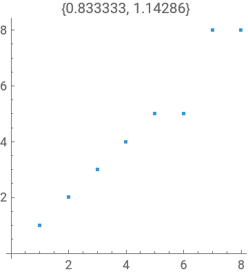
Recall that we looked at the picture below and immediately conjectured that the slopes formed by the lines from the origin to the points obeyed k<y(k)<2k and we found some numerical evidence to support this conjecture.
2
3
In[]:=
Manipulate[ListPlot[y[Range[]],AspectRatio1,ImageSizeSmall],{n,1,6,1},SaveDefinitionsTrue]
n
2
Out[]=
| | ||||||
| |||||||
We will deal with the upper and lower bounds separately. It turns out that the upper bound is easier than the lower bound and we will actually do the upper bound again by a different approach later. It should be mentioned that despite having worked fairly hard to come up with the exact closed form formula below for it doesn’t seem to be helpful to to prove this inequality.
y
y(n)=1+ n-1 ∑ j=1 1 6 IntegerExponent[j,2] (-1) 3+IntegerExponent[j,2] 2 Total[IntegerDigits[j,2]]+1 (-1) |
Theorem: <2 for
y(k)
k
k≥1
Pf: We proceed by induction. We note that and assume that <2 for . We want to show that this is true for so it is sufficient for us to show that this is true for +1≤k≤
y(1)=1
y(k)
k
1≤k≤
n
2
1≤k≤
n+1
2
n
2
n+1
2
|
but it is clear that for so we have
y(k+)≤y(k)+
n
2
n+1
2
1≤k≤
n
2
y(k+ n 2 k+ n 2 |
for which is the same as <2 for +1≤k≤ and we’re done.
1≤k≤
n
2
y(k)
k
n
2
n+1
2
Now we turn to the lower bound and we will need to work a bit harder. By looking at our main graph we can see that all the slopes in the first half of each interval +1≤k≤ are greater than 1, while they are all less than 1 in the second half. This basically comes down to the fact that our underlying permutation is based on reversing but we can show it formally with the following
y(k)
k
n
2
n+1
2
Lemma: For we have for +1≤k≤3 and for
n≥1
y(k)>k
n
2
n-1
2
y(k)<k
3+1≤k≤
n-1
2
n+1
2
Pf:
n 2 n-1 2 | |
n-1 2 | |
n-1 2 | |
n-1 2 |
But this last inequality is clear since the smallest the left side can be is +1 and the largest the right hand side can be is . Similarly we have for as follows
n-1
2
n-1
2
y(k)<k
3+1≤k≤
n-1
2
n+1
2
n-1 2 n+1 2 | |
n-1 2 n 2 | |
n-1 2 n 2 | |
n-1 2 n 2 |
But this last inequality is clear since the largest the left side can be is and the smallest the right hand side can be is +1.
n-1
2
n-1
2
Now we need two lemmas to deal with the quantity . We give a numerical observation and the corresponding proof.
y(k+3)
n-1
2
In[]:=
Block[{n=3},Table[{y[k+3],+y[k]},{k,1,}]]
n-1
2
n
2
n-1
2
Out[]=
{{9,9},{10,10},{12,12},{11,11}}
Lemma: for
y(k+3)=+y(k)
n-1
2
n
2
1≤k≤
n-1
2
Pf: If we have
1≤k≤
n-1
2
|
Again we give a numerical observation and the corresponding proof.
In[]:=
Block[{n=3},Table[{y[k+3],-y[k-]+1},{k,+1,+}]]
n-1
2
n+2
2
n-1
2
n-1
2
n+1
2
n-1
2
Out[]=
{{32,32},{31,31},{29,29},{30,30},{25,25},{26,26},{28,28},{27,27},{17,17},{18,18},{20,20},{19,19},{24,24},{23,23},{21,21},{22,22}}
Lemma: for +1≤k≤+
y(k+3)=-y(k-)+1
n-1
2
n+2
2
n-1
2
n-1
2
n+1
2
n-1
2
Pf: If we have
1≤k-≤
n-1
2
n+1
2
|
So we’re done.
We can now put these two lemmas together if we give up on requiring equality as the following calculation shows
In[]:=
Block[{n=3},Table[{y[k+3],+y[k]},{k,1,}]]
n-1
2
n
2
n+1
2
Out[]=
{{9,9},{10,10},{12,12},{11,11},{32,16},{31,15},{29,13},{30,14},{25,24},{26,23},{28,21},{27,22},{17,17},{18,18},{20,20},{19,19}}
This calculation leads us to the
Conjecture: for
y(k+3)≥y(k)+
n-1
2
n
2
1≤k≤
n+1
2
however we will only prove the following, since it is easier and sufficient for our purposes
Lemma: for
y(k+3)≥y(k)+
n-1
2
n
2
1≤k≤
n
2
Pf: By the above two lemmas we have
y(k+3 n-1 2
|
If we are clearly done. If +1≤k≤ then it follows that . Therefore
1≤k≤
n-1
2
n-1
2
n
2
1≤k-≤
n-1
2
n-1
2
|
Therefore we have
y(k+3 n-1 2
|
and we’re done. Now we can prove the main result.
Theorem: > for
y(k)
k
2
3
k≥1
Pf: The proof is by induction. We assume that > for . We want to show that this is true for , so we need to show it is true for +1≤k≤. By the above comment it is therefore sufficient to show that it is true for . We have the following calculation
y(k)
k
2
3
1≤k≤
n
2
1≤k≤
n+1
2
n
2
n+1
2
3+1≤k≤
n-1
2
n+1
2
|
but the lemma above gives us
y(k+3 n-1 2 k+3 n-1 2 2 3 |
for . This in turn shows that > for . Since =4<5=+3 we’re done.
1≤k≤
n
2
y(k)
k
2
3
3+1≤k≤+3
n-1
2
n
2
n-1
2
n+1
2
n-1
2
n-1
2
n
2
n-1
2
ThueMorse, Evil, Odious, and all that....
ThueMorse, Evil, Odious, and all that....
The title of this section is an homage to the classic book title “Div, Grad, Curl, and all that....”
As I have mentioned before, my intention when I began this effort was that I would only discuss topics in the chronological order in which they were discovered in order to maximize the authenticity of exposition. In the end, this purity was not ideal and not even really all that authentic since one goes back and forth revisiting old approaches in light of new ideas. In particular, it now behooves us to discuss openly what we have nibbling around the edges of: The ThueMorse function which gives the parity of the number of 1’s in the binary representation of an integer. We have already informally defined it, but we now do so formally.
Definition:
ThueMorse(n)=
|
Of course, This can be immediately implemented as
Mod[Total[IntegerDigits[n,2]],2]
Note: Without realizing it, we were effectively working with the ThueMorse idea when we introduced our first version of the position function using the expression
1-
Total[IntegerDigits[n,2]]
(-1)
2
Let’s compare these implementations with the built in ThueMorse function
In[]:=
TableThueMorse[n]==Mod[Total[IntegerDigits[n,2]],2]==,{n,1,32}
1-
Total[IntegerDigits[n,2]]
(-1)
2
Out[]=
{True,True,True,True,True,True,True,True,True,True,True,True,True,True,True,True,True,True,True,True,True,True,True,True,True,True,True,True,True,True,True,True}
This leads to a simple theorem which we don’t need to prove and could just as well have been the definition.
Theorem:
ThueMorse(n)= 1- Total[IntegerDigits[n,2]] (-1) 2 |
According to Wikipedia, Conway is credited with the terms Odious and Evil. Odious numbers have ThueMorse values of 1 and Evil numbers have ThueMorse values of 0. Here are some evil numbers.
In[]:=
Select[Range[32],ThueMorse[#]0&]
Out[]=
{3,5,6,9,10,12,15,17,18,20,23,24,27,29,30}
Since these terms are inspired by even and odd, in other words parity, but have a negative connotation we will call this quality pariahity. See what I did there? It’s clever, yes? I have no idea if it is original. Was it really cleverness though? Nope. All I did was the following.
In[]:=
pariWords=DictionaryLookup["pari"~~___]
Out[]=
{pariah,pariahs,parietal,parimutuel,parimutuels,paring,parings,parish,parishes,parishioner,parishioners,parities,parity}
As luck would have it, the first word has negative connotations! It’s kind of fantastic how much knowledge is “at the ready” in the Wolfram Language and it goes way beyond merely having a dictionary available. On a related note, sometimes I wonder if the reason some people complain about the Wolfram language is that people who like it are constantly going on and on about how great it is.
Anyway, now we are ready for a slogan:
Everything we are doing comes down to parity and pariahity.
Slogans are fun, but I just put that bold slogan there in a shameless effort to promote my new word. In the course of trying to prove more advanced results we gained a sense of what we needed to be true about ThueMorse and then ran some calculations to verify that the statements were true as follows.
In[]:=
Table[ThueMorse[k-1]==1-ThueMorse[2k-1],{k,1,16}]
Out[]=
{True,True,True,True,True,True,True,True,True,True,True,True,True,True,True,True}
In[]:=
Table[ThueMorse[2k+1]==1-ThueMorse[2k],{k,1,16}]
Out[]=
{True,True,True,True,True,True,True,True,True,True,True,True,True,True,True,True}
In[]:=
Table[IntegerExponent[n,2]+Total[IntegerDigits[n,2]]==Total[IntegerDigits[n-1,2]]+1,{n,1,16}]
Out[]=
{True,True,True,True,True,True,True,True,True,True,True,True,True,True,True,True}
Then because we are doing math we formulate the statement precisely and prove them. We will need these lemmas shortly.
Lemma:
Pf: The first statement is clear since if the binary representation of, then the representation of is .
Total[IntegerDigits[2n+1,2]]+1=Total[IntegerDigits[n,2]]+1
Pf: The first statement is clear since if the binary representation of
nis{,,...,}
b
n
b
n-1
b
0
2n+1
{,,...,,1}
b
n
b
n-1
b
0
Lemma:
Pf: This statement just follows from the above by replacing with .
Total[IntegerDigits[2n-1,2]]+1=Total[IntegerDigits[n-1,2]]
Pf: This statement just follows from the above by replacing
n
n-1
Lemma:
Pf: This statement is slightly more substantial. There are two cases: odd and even. If is odd, it ends in a 1 and it is clear that since and all you did on the right hand side was add and subtract 1. If is even it ends in some number, say , of consecutive 0’s and suppose it has 1’s before those 0’s. Therefore the LHS is . On the other hand, when you subtract 1 from the zeros become 1’s but you lose one of the ones resulting in a number with 1’s. Therefore the RHS is and we’re done.
IntegerExponent[n,2]+Total[IntegerDigits[n,2]]=Total[IntegerDigits[n-1,2]]+1
Pf: This statement is slightly more substantial. There are two cases:
n
n
n
IntegerExponent[n,2]+Total[IntegerDigits[n,2]]=Total[IntegerDigits[n-1,2]]+1
IntegerExponent[n,2]=0
n
k
j
k+j
n
k
k
j+k-1
j+k
A Different Approach to y
A Different Approach to
y
As we’ve seen, the position function turns out to have many hidden patterns. When we plot it is a fractal graph but it seems to be deviating from a line in a quasi random but also in a slightly increasing way on average. Staying in the deterministic realm, we ask the following question: to what extent is deviating from linearity with respect to multiplying by 2? This is a possible narrative that might lead to the calculations below.
y
y
Comment: This is not how we came to conjecture the results below, but such “false” or “possible” discovery narratives or histories are nonetheless useful as a means of connecting ideas. This is not my idea and is straight from Polya in his book “Mathematical Discovery” where he compares mathematical pedagogy to biology citing the biological principle of “phylogeny recapitulates ontogeny” as a model for how to best teach students: give them some idea of the genesis and history of the ideas! In other words, do the exact opposite of what sometimes used to be fashionable in math classrooms: present the slickest possible modern definition first, and then show that the classical results are special cases. This may be logically efficient, but it is pedagogically “bass-ackwards”, as my dad used to say, and has never worked very well except perhaps for maybe a small and very select few. In short, if you’re going to talk about classical examples anyway--and you should-- for god’s sake do them first! This comment may not be necessary since “Bourbakism” seems to have fallen out of favor.
Follow up Comment: It has always struck me as so stupid to present the most abstract approach first that I have a rather paranoid theory about it: Some mathematicians see it as their duty to “weed out” those they perceive as unworthy. Ironically, these self appointed “guardians of excellence” are often not really such great mathematicians themselves--the great ones are probably thinking about math I imagine. I’ve known a few faculty that seemed to approach this “duty” with genuine gusto. Not surprisingly, the “weeds” often end up being the “under-represented” minorities and women, but I’ve actually known a few white male mathematicians who have recounted with real bitterness the gratuitous weed out efforts they were forced to endure. Anyway, my paranoid theory is that this sort of obviously terrible approach to teaching facilitates the culling process.
Follow up to the follow up comment: The above comment begs the obvious question: how was it that I survived the culling process? Many attempts were made. The short answer is that my parents, particularly my mother, did their jobs well. Also, a few of my early teachers and mentors played a significant role. By the time I arrived at the university, I was simply too strong to be culled. Some have called it arrogance I’m sure, another term, I believe, is “uppity”. It’s actually just hard won confidence. The faculty that do this sort of thing have no problem crushing the dreams of interested students by bluntly and gratuitously telling them to their face, “You don’t have what it takes to be a mathematician” for example. I never heard this one exactly, but I heard something similar and a bit more amusing. Of course, when directed at a fragile student, these assessments -- which, in the new terminology, are really micro-aggressions -- become self fulfilling prophecies. They are almost always done in private, so there is no evidence other than the word of the now broken student. Finally, to add insult to injury, you sometimes have to listen to the perpetrators of these crimes lamenting, “If only there were a pipeline” or, even more outrageously, accepting awards for their teaching and dedication to students. Perhaps it would make more sense if the award was for their dedication to “some” students. All of this phoniness sort of makes me want to vomit actually.
Anyway, returning to mathematics, consider the calculations below. We discovered them by considering and first of course.
y(2n)-2y(n)
y(2n+1)-2y(n+1)
In[]:=
Tabley[2n],2y[n]-,{n,1,32}
1-
Total[IntegerDigits[n-1,2]]
(-1)
2
Out[]=
{{2,2},{3,3},{7,7},{6,6},{15,15},{14,14},{10,10},{11,11},{31,31},{30,30},{26,26},{27,27},{18,18},{19,19},{23,23},{22,22},{63,63},{62,62},{58,58},{59,59},{50,50},{51,51},{55,55},{54,54},{34,34},{35,35},{39,39},{38,38},{47,47},{46,46},{42,42},{43,43}}
In[]:=
Tabley[2n+1],2y[n+1]-,{n,1,32}
1-
Total[IntegerDigits[2n+1,2]]
(-1)
2
Out[]=
{{4,4},{8,8},{5,5},{16,16},{13,13},{9,9},{12,12},{32,32},{29,29},{25,25},{28,28},{17,17},{20,20},{24,24},{21,21},{64,64},{61,61},{57,57},{60,60},{49,49},{52,52},{56,56},{53,53},{33,33},{36,36},{40,40},{37,37},{48,48},{45,45},{41,41},{44,44},{128,128}}
Note: It is worth noting that the expression is related to a larger pattern, for lack of a better word, you see in mathematics constantly: the commutator. You have two operations/functions and you perform them in different orders. When you get the same result we say the operations are commutative and non-commutative otherwise. We are speaking a bit loosely here since the commutator concept comes up in various algebraic settings, and in this case we have the ring version where the multiplication is function composition and the other operation is pointwise addition of functions. Non commutative means more complicated, but mathematicians like to turn these situations into opportunities because it also means things are more interesting! Why? Because it then makes sense to measure the deviation from commutativity. In our current case we have two functions: “multiply by 2” and . Apparently, they almost commute but not quite and the correction term is quite interesting. As a point of reference this is similar to the computation of the Lie bracket of two vector fields in differential geometry.
y(2n)-2y(n)
y
Comment: I first learned about conjugation from the article Douglas Hofstader wrote on the Rubik’s cube in Scientific American. A friend of mine told me that you could learn to come up with your own solving algorithm by following the ideas in this article. Those ideas are group theory in general and conjugation in particular. He is also the one who told me about the Ross program which plays a significant role in the approach I have adopted in this monograph. One conclusion to draw from this comment is that it is important for nerds to have some nerd friends. An additional possible conclusion is that “nerd” schools, or at least schools with a vibrant nerd culture, are important for the intellectual development of nerds. Finally, I would suggest that the people involved in running nerd schools should either be nerds or former nerds themselves or at least have strong nerd sympathies. Otherwise it all becomes a diluted mess and standards inevitably get lowered to the point that all you have is just another decent school -- what a waste! But it would now appear that we are going off on a tangent. That was a very bad nerd joke.
Comment: I am quite sure there are those that will take umbrage at my “diluted” comment, since I am unapologetically advocating for the notion that students with advanced training and interest in mathematics should have the opportunity to be grouped together. In truth, I actually don’t like the phrase “ability grouping” but I do like the phrase I made up “preparation and interest grouping” however. In my mind, the historical problems with academic tracking were the correlations based on race and class caused by racism and classicism. If these causes and correlations are removed, it strikes me as common sense that having students with similar preparations and interests grouped together makes for a better teaching environment. Apparently this is a controversial position but everyone regards it as perfectly normal that many college campuses have athletic dorms for the “student-athletes”.
Comment: That’s another thing I don’t get. When I was a kid nobody used the term “student-athletes”. It’s as though, over time, a new class has been defined using multiple inheritance. Everyone says that “student-athletes” are students first, suggesting that it is a derived class, but the instantiated objects of the student-athlete class seem to have additional methods not present in either parent class in my experience.
Comment: Measuring “ability” by using a number produced by a test is problematic and suffers from the “reification” fallacy: how do you measure “ability”? The answer is usually given tautologically as “That number which my test produces” and, by false implication, it is genetic and fixed. I encountered these ideas in the excellent but poorly named book, “The Mismeasure of Man” by Stephen J. Gould, among other sources, but in the modern terminology this is now called “fixed-mindset” thinking and everybody in education mentions this phrase constantly and obligatorily.
Comment: The above discussions that I am having with myself reminds me of the philosopher Neil Postman’s discussions regarding the importance of language in which he cites Orwell’s 1984: suddenly verboten words, new words, new meanings to old words, etc... be suspicious! It suggests that we should all run self-diagnostics like Data does in TNG to make sure our language “symbol tables” have not been altered against our will.
Returning to the mathematical narrative, the above calculation gives us a conjecture we could call the “almost 2-linearity” of .
y
Note: We will do something a little bit different with this result. We will do the proof entirely using Mathematica’s input mode. We have alluded to traditional math vs computer code issues before, and this time we won’t do some computations and then type it up as text, we’ll just leave it all as code! You could call it “mathcode” or something but it already has a name: the Wolfram language of course! I’m not just being cute here, math formulas, properly written are legitimate Wolfram language statements whereas it would be quite difficult to write the argument below in C++ or Java. Despite writing the argument in code, it’s still a legitimate proof however since the code will be identical to what we would have written or typed. We tend to do this when we make mistakes and get confused (which happened) and then we erase all evidence of the struggle, but I want to show you how you can use Mathematica as an incredibly effective scratch pad once you get comfortable with it. This technique is particularly useful if you find that you are algebraically challenged or fearful of objects like summations. I mention this because I have had many students who either paid no attention or learned very little from their math classes in high school and then discover that they are interested in computer science--which is wonderful--but then they learn, to their chagrin, that they really do need to be good at algebra, manipulating summations, induction, and recursion in their theoretical computer science/discrete math courses.
We now prove our
Conjecture:
|
Note: This will be long but each step is elementary, and when the step is not clear, I will explain it.
Pf: First we deal with . We have the following expression
y(2n)
y(2n)=1+ 2n-1 ∑ j=1 1 6 IntegerExponent[j,2] (-1) 3+IntegerExponent[j,2] 2 Total[IntegerDigits[j,2]]+1 (-1) |
We now switch to Wolfram language code. Again, we are doing exactly the steps we would do in a traditional proof, we are simply doing it in input mode rather than in a math text cell so that we can check our work as we go.
In[]:=
Tabley[2n],1+-3++,{n,1,10}
2n-1
∑
j=1
1
6
IntegerExponent[j,2]
(-1)
IntegerExponent[j,2]+3
2
Total[IntegerDigits[j,2]]+1
(-1)
Out[]=
{{2,2},{3,3},{7,7},{6,6},{15,15},{14,14},{10,10},{11,11},{31,31},{30,30}}
Now we break the sum up into even and odd terms.
In[]:=
Tabley[2n],1+-3+++-3++,{n,1,10}
n-1
∑
j=1
1
6
IntegerExponent[2j,2]
(-1)
IntegerExponent[2j,2]+3
2
Total[IntegerDigits[2j,2]]+1
(-1)
n
∑
j=1
1
6
IntegerExponent[2j-1,2]
(-1)
IntegerExponent[2j-1,2]+3
2
Total[IntegerDigits[2j-1,2]]+1
(-1)
Out[]=
{{2,2},{3,3},{7,7},{6,6},{15,15},{14,14},{10,10},{11,11},{31,31},{30,30}}
Since is 0 the second summation simplifies.
IntegerExponent[2j-1,2]
In[]:=
Tabley[2n],1+-3+++,{n,1,10}
n-1
∑
j=1
1
6
IntegerExponent[j,2]+1
(-1)
IntegerExponent[j,2]+4
2
Total[IntegerDigits[j,2]]+1
(-1)
n
∑
j=1
Total[IntegerDigits[2j-1,2]]+1
(-1)
Out[]=
{{2,2},{3,3},{7,7},{6,6},{15,15},{14,14},{10,10},{11,11},{31,31},{30,30}}
We “peel off” a term and put it into a separate summation.
IntegerExponent[j,2]+3
2
In[]:=
Tabley[2n],1+-3+++()+,{n,1,10}
n-1
∑
j=1
1
6
IntegerExponent[j,2]+1
(-1)
IntegerExponent[j,2]+3
2
Total[IntegerDigits[j,2]]+1
(-1)
n-1
∑
j=1
1
6
IntegerExponent[j,2]+3
2
Total[IntegerDigits[j,2]]+1
(-1)
n
∑
j=1
Total[IntegerDigits[2j-1,2]]+1
(-1)
Out[]=
{{2,2},{3,3},{7,7},{6,6},{15,15},{14,14},{10,10},{11,11},{31,31},{30,30}}
We change to by adding a correction term and then we substitute y[n]
IntegerExponent[j,2]+1
(-1)
IntegerExponent[j,2]
(-1)
In[]:=
Tabley[2n],y[n]+-+()+,{n,1,10}
n-1
∑
j=1
1
6
IntegerExponent[j,2]+1
(-1)
IntegerExponent[j,2]
(-1)
Total[IntegerDigits[j,2]]+1
(-1)
n-1
∑
j=1
1
6
IntegerExponent[j,2]+3
2
Total[IntegerDigits[j,2]]+1
(-1)
n
∑
j=1
Total[IntegerDigits[2j-1,2]]+1
(-1)
Out[]=
{{2,2},{3,3},{7,7},{6,6},{15,15},{14,14},{10,10},{11,11},{31,31},{30,30}}
Now we add more correction terms to create another copy of .
y(n)-1
In[]:=
Tabley[2n],y[n]+-+3-+-3+++,{n,1,10}
n-1
∑
j=1
1
6
IntegerExponent[j,2]+1
(-1)
IntegerExponent[j,2]
(-1)
IntegerExponent[j,2]
(-1)
Total[IntegerDigits[j,2]]+1
(-1)
n-1
∑
j=1
1
6
IntegerExponent[j,2]
(-1)
IntegerExponent[j,2]+3
2
Total[IntegerDigits[j,2]]+1
(-1)
n
∑
j=1
Total[IntegerDigits[2j-1,2]]+1
(-1)
Out[]=
{{2,2},{3,3},{7,7},{6,6},{15,15},{14,14},{10,10},{11,11},{31,31},{30,30}}
Now we make the substitution and simplify the summation containing the correction terms
y[n]
In[]:=
Tabley[2n],2y[n]-1+3+3+,{n,1,10}
n-1
∑
j=1
1
6
IntegerExponent[j,2]+1
(-1)
Total[IntegerDigits[j,2]]+1
(-1)
n
∑
j=1
Total[IntegerDigits[2j-1,2]]+1
(-1)
Out[]=
{{2,2},{3,3},{7,7},{6,6},{15,15},{14,14},{10,10},{11,11},{31,31},{30,30}}
We further simplify the summation containing the correction terms and distribute the term
Total[IntegerDigits[j,2]]+1
(-1)
In[]:=
Tabley[2n],2y[n]-1+++,{n,1,10}
1
2
n-1
∑
j=1
IntegerExponent[j,2]+Total[IntegerDigits[j,2]]
(-1)
Total[IntegerDigits[j,2]]+1
(-1)
n
∑
j=1
Total[IntegerDigits[2j-1,2]]+1
(-1)
Out[]=
{{2,2},{3,3},{7,7},{6,6},{15,15},{14,14},{10,10},{11,11},{31,31},{30,30}}
Now we use our lemmas and
Total[IntegerDigits[2j-1,2]]+1=Total[IntegerDigits[j-1,2]]
IntegerExponent[j,2]+Total[IntegerDigits[j,2]]=Total[IntegerDigits[j-1,2]]+1
In[]:=
Tabley[2n],2y[n]-1+++,{n,1,10}
1
2
n-1
∑
j=1
Total[IntegerDigits[j-1,2]]+1
(-1)
Total[IntegerDigits[j,2]]+1
(-1)
n
∑
j=1
Total[IntegerDigits[j-1,2]]
(-1)
Out[]=
{{2,2},{3,3},{7,7},{6,6},{15,15},{14,14},{10,10},{11,11},{31,31},{30,30}}
Now we move the last summation into the first summation leaving the last leftover term at the end. Remember the factor of .
1
2
In[]:=
Tabley[2n],2y[n]-1+++,{n,1,10}
1
2
n-1
∑
j=1
Total[IntegerDigits[j-1,2]]
(-1)
Total[IntegerDigits[j,2]]+1
(-1)
Total[IntegerDigits[n-1,2]]
(-1)
Out[]=
{{2,2},{3,3},{7,7},{6,6},{15,15},{14,14},{10,10},{11,11},{31,31},{30,30}}
We pull a factor of out of the summation. You probably are beginning to see where we are going.
-1
In[]:=
Tabley[2n],2y[n]-1--+,{n,1,10}
1
2
n-1
∑
j=1
Total[IntegerDigits[j,2]]
(-1)
Total[IntegerDigits[j-1,2]]
(-1)
Total[IntegerDigits[n-1,2]]
(-1)
Out[]=
{{2,2},{3,3},{7,7},{6,6},{15,15},{14,14},{10,10},{11,11},{31,31},{30,30}}
That’s right! You guessed it telescoping sums again!!!! After this, it’s clear sailing. By the way, the reason you could see that telescoping sums might be coming is simple: how else were we going to get rid of the summation?
In[]:=
Tabley[2n],2y[n]-1--+,{n,1,10}
1
2
Total[IntegerDigits[n-1,2]]
(-1)
Total[IntegerDigits[0,2]]
(-1)
Total[IntegerDigits[n-1,2]]
(-1)
Out[]=
{{2,2},{3,3},{7,7},{6,6},{15,15},{14,14},{10,10},{11,11},{31,31},{30,30}}
In[]:=
Tabley[2n],2y[n]--+,{n,1,10}
1
2
1
2
Total[IntegerDigits[n-1,2]]
(-1)
Total[IntegerDigits[n-1,2]]
(-1)
Out[]=
{{2,2},{3,3},{7,7},{6,6},{15,15},{14,14},{10,10},{11,11},{31,31},{30,30}}
In[]:=
Tabley[2n],2y[n]-+,{n,1,10}
1
2
1
2
Total[IntegerDigits[n-1,2]]
(-1)
Out[]=
{{2,2},{3,3},{7,7},{6,6},{15,15},{14,14},{10,10},{11,11},{31,31},{30,30}}
In[]:=
Tabley[2n],2y[n]-,{n,1,10}
1-
Total[IntegerDigits[n-1,2]]
(-1)
2
Out[]=
{{2,2},{3,3},{7,7},{6,6},{15,15},{14,14},{10,10},{11,11},{31,31},{30,30}}
So we have shown that
y(2n)=2y(n)- 1- Total[IntegerDigits[n-1,2]] (-1) 2 |
Now we want to deal with . We could repeat what we just did but let’s instead leverage the previous result and we’ll just write this out in a traditional manner. Since we have
y(2n+1)
y(n)=1+ n-1 ∑ j=1 1 6 IntegerExponent[j,2] (-1) 3+IntegerExponent[j,2] 2 Total[IntegerDigits[j,2]]+1 (-1) |
It follows that
y(2n+1)-y(2n)= 1 6 IntegerExponent[2n,2] (-1) 3+IntegerExponent[2n,2] 2 Total[IntegerDigits[2n,2]]+1 (-1) |
Therefore we can simplify by the sequence of steps below
y(2n+1)
|
Now we use our result
y(2n)
2y(n)- 1- Total[IntegerDigits[n-1,2]] (-1) 2 1 6 IntegerExponent[2n,2] (-1) 3+IntegerExponent[2n,2] 2 Total[IntegerDigits[2n,2]]+1 (-1) |
but we also have
y(n+1)-y(n)= 1 6 IntegerExponent[n,2] (-1) 3+IntegerExponent[n,2] 2 Total[IntegerDigits[n,2]]+1 (-1) |
which gives
2y(n)=2y(n+1)- 1 6 IntegerExponent[n,2] (-1) 4+IntegerExponent[n,2] 2 Total[IntegerDigits[n,2]]+1 (-1) |
Therefore we can continue the simplification of as follows
y(2n+1)
2y(n+1)- 1 6 IntegerExponent[n,2] (-1) 4+IntegerExponent[n,2] 2 Total[IntegerDigits[n,2]]+1 (-1) 1- Total[IntegerDigits[n-1,2]] (-1) 2 1 6 IntegerExponent[2n,2] (-1) 3+IntegerExponent[2n,2] 2 Total[IntegerDigits[2n,2]]+1 (-1) |
which is the same as
2y(n+1)+ 1 6 IntegerExponent[n,2] (-1) 4+IntegerExponent[n,2] 2 Total[IntegerDigits[n,2]]+1 (-1) 1- Total[IntegerDigits[n-1,2]] (-1) 2 1 6 IntegerExponent[n,2] (-1) 4+IntegerExponent[n,2] 2 Total[IntegerDigits[n,2]]+1 (-1) |
which simplifies to
2y(n+1)+ 1- IntegerExponent[n,2] (-1) 2 Total[IntegerDigits[n,2]]+1 (-1) 1- Total[IntegerDigits[n-1,2]] (-1) 2 |
which is equivalent to
2y(n+1)+ Total[IntegerDigits[n,2]]+1 (-1) IntegerExponent[n,2]+Total[IntegerDigits[n,2]]+1 (-1) 2 1- Total[IntegerDigits[n-1,2]] (-1) 2 |
2y(n+1)+ Total[IntegerDigits[n,2]]+1 (-1) Total[IntegerDigits[n-1,2]] (-1) 2 1- Total[IntegerDigits[n-1,2]] (-1) 2 |
2y(n+1)+ Total[IntegerDigits[n,2]]+1 (-1) 2 |
Now we use our lemma to give us
Total[IntegerDigits[n,2]]+1=Total[IntegerDigits[2n+1,2]]+1
2y(n+1)- 1- Total[IntegerDigits[2n+1,2]] (-1) 2 |
And we’re done! We strongly, suspect that there must be an easier way to do this but when you don’t see a clever path, it’s time to just roll up your sleeves and grind it out.
Using the definition ThueMorse, we immediately have the following corollary
Corollary:
|
Our goal now is not to be exhaustive but to show how this new perspective on can be used to obtain additional results.
y
We can also use these formulas to create a different recursive formulation for ,
y
Corollary: is given by the following recursive scheme
y
y(1)=1 | ||||||
y(n)=
|
Since we can implement this as follows but we will use in place of .
ThueMorse[n-2]=ThueMorse2-1
n
2
yy
y
In[]:=
Clear[yy]
In[]:=
yy[1]=1;
In[]:=
yy[n_/;OddQ[n]]:=2yy-ThueMorse[n];yy[n_/;EvenQ[n]]:=2yy-ThueMorse[n-2];
n+1
2
n
2
In[]:=
Table[{y[n],yy[n]},{n,1,32}]
Out[]=
{{1,1},{2,2},{4,4},{3,3},{8,8},{7,7},{5,5},{6,6},{16,16},{15,15},{13,13},{14,14},{9,9},{10,10},{12,12},{11,11},{32,32},{31,31},{29,29},{30,30},{25,25},{26,26},{28,28},{27,27},{17,17},{18,18},{20,20},{19,19},{24,24},{23,23},{21,21},{22,22}}
This form of our recursive formulation for immediately gives us a one line recursive definition for completely different from our previous one line definition. What is nice about this is that it nicely encapsulates the fact that everything about these investigations keeps coming back to doubling/halving and parity/pariahity.
y
y
Corollary: is given by the following recursive scheme
y
|
Pf: Just use the above formulation and the fact that
1+=
Mod[n,2]
(-1)
|
|
We can implement this as follows but we will use in place of .
yyy
y
In[]:=
Clear[yyy]
In[]:=
yyy[1]=1;yyy[n_]:=2yyyCeiling-ThueMorse[n-1-];
n
2
Mod[n,2]
(-1)
In[]:=
Table[{y[n],yyy[n]},{n,1,32}]
Out[]=
{{1,1},{2,2},{4,4},{3,3},{8,8},{7,7},{5,5},{6,6},{16,16},{15,15},{13,13},{14,14},{9,9},{10,10},{12,12},{11,11},{32,32},{31,31},{29,29},{30,30},{25,25},{26,26},{28,28},{27,27},{17,17},{18,18},{20,20},{19,19},{24,24},{23,23},{21,21},{22,22}}
As you can see we have gotten a great deal of mileage out of the above corollary. Now we will use it to do something different. Rather than use it to create yet another recursive formula for computing , we will pull things apart to improve our basic understanding. You may have noticed that the terms odious and evil bare more than a little resemblance to odd and evil. Obviously, this is not an accident, yet we really did dot not know what the connection was between these notions! In the course of our investigations we made a “discovery” which answered this question. It is actually a bit shocking how long it took for me to clearly formulate this. Observe the following table
y
In[]:=
Table[{{k-1,If[ThueMorse[k-1]1,"odious","evil"]},{y[k],If[Mod[y[k],2]1,"odd","even"]}},{k,1,16}]//Column
Out[]=
{{0,evil},{1,odd}} |
{{1,odious},{2,even}} |
{{2,odious},{4,even}} |
{{3,evil},{3,odd}} |
{{4,odious},{8,even}} |
{{5,evil},{7,odd}} |
{{6,evil},{5,odd}} |
{{7,odious},{6,even}} |
{{8,odious},{16,even}} |
{{9,evil},{15,odd}} |
{{10,evil},{13,odd}} |
{{11,odious},{14,even}} |
{{12,evil},{9,odd}} |
{{13,odious},{10,even}} |
{{14,odious},{12,even}} |
{{15,evil},{11,odd}} |
Which leads to the following conjecture/theorem
Theorem: is odious/evil iff is even/odd respectively.
k-1
y(k)
Pf: First we recall our two properties
|
Then we apply Mod[ ,2] and some ThueMorse properties
|
So
|
Therefore we have shown that the following parity/pariahity identity
|
and our theorem follows.
In other words the connection between odd/even and odious/evil is the function ! This is pretty funny if you think about it: we’ve been trying to understand and we also wanted to know what the connection was between parity and pariahity and it’s almost the same question! Hilarious. These jokes write themselves.
y
y
If we re-write our identity as
-ThueMorse[k-1] then we are really saying that the diagram below commutes
Mod[y(k),2]=1 |

In[]:=
Table[Mod[y[n],2]1-ThueMorse[n-1],{n,-16,16}]
Out[]=
{True,True,True,True,True,True,True,True,True,True,True,True,True,True,True,True,True,True,True,True,True,True,True,True,True,True,True,True,True,True,True,True,True}
Comment: I had an analysis professor that used to love to announce during lectures that “the diagram commutes!” for the most trivial observations. It was a good natured joke making fun of my interest in algebraic topology. Honestly, I thought it was funny, but I never convinced him that commutative diagrams can actually be useful if the categories have non-trivial functors acting on them.
Note: The above diagram is essentially a visual representation of the parity/pariahity connection. We say that “solves” the diagram, but it is clear that is not the unique solution since we can add even numbers willy nilly to the output of without changing the parity. Therefore is not really “the” connection but merely “a” connection between parity and pariahity. Finally, we concede that the use of a “commutative diagram here is more just to give a nice clear visual representation of the the above equation and we have no plans to hit the diagram with any cool functors.
y
y
y
y
Note that we can re-write the above identity as follows
|
Since ThueMorse is even this shows that must be even as well which is not a surprise since we already knew that is even. Finally, with a little more algebra, we can re-write this identity--also called the parity/pariahity identity-- one last time as follows
Mod[y(k+1),2]
y(k+1)
|
In words, this says that the map ThueMorse(k) and Mod[k ,2] are essentially the same “up to a conjugation of by translation”. Which can be written as
y
Theorem: is even/odd iff is evil/odious.
y(k+1)-1
k
But wait there’s more!
But wait there’s more!
If there is one result that summarizes the whole halving/doubling, parity/pariahity it is the following formula
y(n)=2yCeiling n 2 Mod[n,2] (-1) |
We can derive two facts from this statement
|
and we have
|
Therefore we have
y(n) 2 n 2 1+y(n) 2 |
which we can re-write two ways and we call both doubling/halving identities
yCeiling n 2 y(n) 2 |
y(n)≤2yCeiling n 2 |
Moreover, since all the number are integers and this is the same as
1-ThueMorse[k-1]==Mod[y[k],2]
y(n)=
|
We can implement the above as yet another recursive scheme for computing . We will use in place of .
y
z
y
In[]:=
Clear[z]
In[]:=
z[1]=1;z[n_]:=IfThueMorse[n-1]0,2zCeiling-1,2zCeiling;
n
2
n
2
In[]:=
Table[z[k],{k,1,32}]
Out[]=
{1,2,4,3,8,7,5,6,16,15,13,14,9,10,12,11,32,31,29,30,25,26,28,27,17,18,20,19,24,23,21,22}
Finally, we can express the doubling/halving identity in terms of a commutative diagrams which is kind of cute.

In[]:=
TableyCeiling==Ceiling,{n,1,32}
n
2
y[n]
2
Out[]=
{True,True,True,True,True,True,True,True,True,True,True,True,True,True,True,True,True,True,True,True,True,True,True,True,True,True,True,True,True,True,True,True}
Note: This diagram is essentially a visual representation of the whole doubling/halving aspect of our problem. Again, “solves the diagram” but this requirement alone doesn’t force a unique solution. Clearly, there will always be two possible choices to make at every step leading to many possible solutions. Fortunately, this choice is determined by the parity of which is exactly what we have specified by the above formula/diagram. We therefore now have a simple characterization of .
y
y(k)
y
Theorem: is the unique simultaneous solution to both of the above diagrams.
y
A Generalization
A Generalization
Comment: Mathematicians specialize in generalizing. Unfortunately, this seems to annoy some students and frankly even some mathematicians. They seem to feel as though mathematicians generalize merely for it’s own sake or perhaps just to make things maximally confusing so as few people as possible want to study mathematics. Actually, the point and value of generalizing, in addition to widening the applicability of results obviously, is to make things simpler and clearer to facilitate understanding. Despite this, the most general framework is almost certainly not the most pedagogically appropriate for a first encounter.
Now we have had quite a few approaches to and each had it’s charms, strengths and weaknesses. It really depends on what you want to do or understand that determines which is better in a given situation. For example, the mapping problem approach makes it clear that we can decouple the problem into two parts, the doubling/halving and the parity/pariahity, and it is the interaction of both of these properties that produces the interesting behavior of and this makes the mapping approach an easy candidate for generalization.
y
y
That said, generalizing involves making choices and if you allow too much flexibility you can’t really prove anything interesting. For example, there is not much we can say about an arbitrary map. We choose to leave the doubling/halving property intact, but we will generalize the parity/pariahity property. More precisely, we now suppose that , not necessarily , obeys our doubling/halving property. We now need some scheme by which to choose the parity of at each step. In other words, we need a predicate function, say parityScheme, to determine the parity of . This gives us the following set up for .
z
y
z
z
z
z(n)=
|
All we need to do is take the above recursive code and wrap it in Manipulate replacing the parity scheme based on pariahity with our predicate predicateScheme which we can vary. We will also very crudely measure the growth rate of the various outputs by looking at the maximum and minimum slope of the lines determined by the points with the origin.
In[]:=
ManipulateModule{z,data,slopes,max,min},z[1]=1;z[n_]:=IfparityScheme[n],2zCeiling-1,2zCeiling;data=Table[{k,z[k]},{k,1,}];slopes=data/.{p_,q_};{max,min}=N[{Max[slopes],Min[slopes]}];ListPlot[data,AspectRatio1,PlotLabel{min,max},ImageSizeSmall],{m,2,6,1},{parityScheme,{##&,ThueMorse[#-1]1&,ThueMorse[#]1&,EvenQ,OddQ,ThueMorse[#]0&,ThueMorse[#-1]0&,##+1&}},SaveDefinitionsTrue
n
2
n
2
m
2
q
p
Out[]=
| | ||||||||
| |||||||||
The pure functions listed are simply various, parity choosing schemes. We have ordered them roughly in terms of size as measured by our “slope norm”. Here is quick catalog of these schemes.
◼
##& , always true, all are odd, the smallest
z(n)
◼
ThueMorse[#-1]1&, bitwise complement of the usual scheme, is even/odd iff is evil/odious
z(k)
k-1
◼
ThueMorse[#]1&, bitwise complement of shifted usual scheme, is even/odd iff is evil/odious
z(k)
k
◼
EvenQ, even gives odd.
n
z(n)
◼
OddQ, odd gives odd, identity, 1-1
n
z(n)
◼
ThueMorse[#]0&, shifted usual scheme, is even/odd iff is odious/evil.
z(k)
k
◼
ThueMorse[#-1]0&, usual scheme, is even/odd iff is odious/evil, 1-1
z(k)
k-1
y
◼
##+1&, always false, all are even, the largest
z(n)
Turning the parity scheme into a variable has enabled us to see how the doubling/halving identity and the parity scheme interact to produce a variety of growth behaviors, but you probably noticed that the growth never exceeded 2. In other words, the doubling halving identity appears to impose some control on the growth of any function which obeys it. Recall that we had already noticed this for when we conjectured in the geometry section when we noticed that the slopes of the lines formed by the points of our main graph that the slopes of the lines determined by our points in the graph we all between and 2. It looks like the lower bound really does depend on , but the upper bound is apparently more general.
y
y
2
3
y
We now consider a few of these schemes in greater detail. The “extreme” parity schemes are the first one “all are odd” and the last one “all are even”. It’s clear that “all are odd” produces the smallest values.
z(n)
z(n)
z(n)
In[]:=
z[1]=1;z[n_]:=2zCeiling-1;Table[z[k],{k,1,16}]
n
2
Out[]=
{1,1,1,1,1,1,1,1,1,1,1,1,1,1,1,1}
The solution to this recursion is clearly and this could be proven easily by induction. On the other hand, it’s clear that “all are even” produces the largest values and we can see them easily as follows.
z(n)=1
z(n)
In[]:=
z[1]=1;z[n_]:=2zCeiling;Table[z[k],{k,1,16}]
n
2
Out[]=
{1,2,4,4,8,8,8,8,16,16,16,16,16,16,16,16}
The solution to this recursion is which we can see as follows
z(n)=
Ceilling[(n)]
lg
2
2
In[]:=
Table[,{k,1,16}]
Ceiling[Log2[k]]
2
Out[]=
{1,2,4,4,8,8,8,8,16,16,16,16,16,16,16,16}
We will prove this by induction below but first we’ll discuss some of the intermediate schemes. Obviously there are many possible parity schemes in between these extreme cases. Two come to mind immediately: ThueMorse[#-1]0& which has been virtually the entire focus of this monograph and OddQ which produces the identity. We can see this easily as follows. Using OddQ comes down to
z(n)=
|
In[]:=
z[1]=1;z[n_]:=IfEvenQ[n],2zCeiling,2zCeiling-1;Table[z[k],{k,1,16}]
n
2
n
2
Out[]=
{1,2,3,4,5,6,7,8,9,10,11,12,13,14,15,16}
By induction, the result follows immediately from the identity .
z(n)=n
2-1=n=2
n+1
2
n
2
Now let’s come back to the upper extreme case parity scheme of “all even”. Despite the simplicity of the situation we will elevate it’s status to that of a theorem. First we need a lemma.
z(n)
Lemma: If +1≤k≤ then .
n
2
n+1
2
CeilingCeiling+1=Ceiling[(k)]
lg
2
k
2
lg
2
Pf: If then we have
If+1≤k≤
n
2
n+1
2
|
which implies
|
On the other hand we also have
|
which gives us
|
so we’re done.
Theorem: If is defined by and then .
z
z(1)=1
z(n)=2zCeiling
n
2
z(n)=
Ceilling[(n)]
lg
2
2
Pf: BWOI. It’s clear true for now assume it is true for all and show that it’s true for +1≤k≤. By the inductive hypothesis and the above lemma we have
k=1
1≤k≤
n
2
n
2
n+1
2
|
and we’re done.
This gives us an immediate corollary since is the largest possible solution we immediately have
z(n)=
Ceilling[(n)]
lg
2
2
z
corollary: if then
zCeiling=Ceiling
n
2
z(n)
2
z(n)≤
Ceilling[(n)]
lg
2
2
This in turn gives us
corollary: if then
zCeiling=Ceiling
n
2
z(n)
2
z(n)<2n
Pf:
z(n)≤=2<2(n)=2n
Ceilling[(n)]
lg
2
2
Ceilling[(n)]-1
lg
2
2
lg
2
2
Note that there is one function which clearly obeys our doubling/halving identity: which is certainly less than . Of course, the application we are interested in is the following
z(n)=n
2n
corollary: If is our position function then
y
y(n)<2n
Note: So we have re-proven our conjecture on the upper bound of the slopes created by our points. We notice again that we have only used the halving doubling property to do this which is why this bound applied to all of our parity schemes. Notice also that the lower bounds varied considerably so the lower bound only applies to which means we will need more than the doubling/halving identity if we want to prove it and indeed we did find it distinctly more difficult to prove than the upper bound.
2
3
y
Computational Issues for y
Computational Issues for
y
We discuss a few timing issues in the computation of our sequence and the differences of .
y
y
Computing y
Computing
y
Let’s see how long it is taking to do these computations by using the Timings function.
In[]:=
timingsRecursive=Module[{y},y[1]=1;y[2]=2;y[j_]:=-y[j-]+1;Table[Timing[y/@Range[];][[1]],{n,1,12}]]
Ceiling[Log2[j]]
2
Ceiling[Log2[j]]-1
2
n
2
Out[]=
{0.00002,0.000085,0.000154,0.000452,0.001313,0.003588,0.008115,0.020185,0.043943,0.255543,0.46343,0.798191}
In[]:=
Ratios[timingsRecursive]
Out[]=
{4.25,1.81176,2.93506,2.90487,2.73267,2.26171,2.48737,2.17701,5.81533,1.81351,1.72236}
Timings depends on your computer and what’s going on in your computer at the time you run it, so it isn’t perfect, but it’s giving us a rough idea that each time we double the data set, the amount of time goes up by a factor between 2 and 3 most of the time for these small data sets.
One might say to oneself, something “like recursion is slow, better to use the closed form formula we developed!”
In[]:=
timingsClosedForm=Module{y},y[1]=1;y[2]=2;y[j_]:=1+-3++;Table[Timing[y/@Range[];][[1]],{n,1,12}]
j-1
∑
k=1
1
6
IntegerExponent[k,2]
(-1)
IntegerExponent[k,2]+3
2
Total[IntegerDigits[k,2]]+1
(-1)
n
2
Out[]=
{0.000025,0.00009,0.000275,0.001026,0.003305,0.015194,0.036268,0.136654,0.56624,2.50231,9.16962,35.5599}
In[]:=
Ratios[timingsClosedForm]
Out[]=
{3.6,3.05556,3.73091,3.22125,4.59728,2.38699,3.76789,4.1436,4.41917,3.66446,3.87801}
This is a disaster! The closed form formula was the key for our theory but it is useless to actually calculate for even these small data sets as it starts out slow and quadruples every time. This should not be a surprise due to the use of the number theoretic functions and the summation.
We can often improve recursion by the use of so-called “dynamic programming” or caching of values. The syntax to tell Mathematica to remember previous results is quite short and simple: we simply add to our recursive definition.
y[j]=
In[]:=
timingsRecursiveCaching=Module[{y},y[1]=1;y[2]=2;y[j_]:=y[j]=-y[j-]+1;Table[Timing[y/@Range[];][[1]],{n,1,12}]]
Ceiling[Log2[j]]
2
Ceiling[Log2[j]]-1
2
n
2
Out[]=
{0.000021,0.000086,0.000111,0.000233,0.000496,0.001712,0.004951,0.006707,0.013473,0.041263,0.071223,0.166701}
In[]:=
Ratios[timingsRecursiveCaching]
Out[]=
{4.09524,1.2907,2.0991,2.12876,3.45161,2.89194,1.35468,2.0088,3.06264,1.72607,2.34055}
This is substantially faster than the recursive version without caching.
In any case the growth in these timings are sufficiently fast that it would therefore behoove us to find a more efficient way to compute this sequence. Fortunately, we don’t have to re-invent the wheel. When we submitted our sequence to OEIS we found the following Wolfram language code from Robert G. Wilson again.
In[]:=
Manipulate[Nest[Join[#,(Length[#]+Range[Length[#],1,-1])[[#]]]&,{1},m],{m,1,8,1},SaveDefinitionsTrue]
Out[]=
| | ||||||
| |||||||
Once again the OEIS site proves to be a marvelous resource which, sadly, I only learned about recently. One nice thing that I noticed in the course of these investigations is that you often find immediately useful Wolfram Language code and sometimes it is the only code present! This shouldn’t be entirely surprising since ease of mathematical manipulation and list processing are deeply embedded in the DNA of the Wolfram language.
We can see that this is much faster than the code we have been using. Note that since we are using pure functions, we don’t need any named variables or scoping constructs
In[]:=
timingsWilsonCode=Table[First@Timing[Nest[Join[#,(Length[#]+Range[Length[#],1,-1])[[#]]]&,{1},n];],{n,1,12}]
Out[]=
{0.000033,0.000014,0.000015,0.000018,0.00002,0.000023,0.000029,0.000032,0.00004,0.000046,0.000109,0.000161}
In[]:=
Ratios[%]
Out[]=
{0.424242,1.07143,1.2,1.11111,1.15,1.26087,1.10345,1.25,1.15,2.36957,1.47706}
This is much faster than our previous methods. Let’s plot all four methods together.
In[]:=
Show[ListLinePlot[timingsRecursive,PlotStyleOrange],ListLinePlot[timingsClosedForm,PlotStyleRed],ListLinePlot[timingsRecursiveCaching,PlotStyleYellow,PlotRangeAll],ListLinePlot[timingsWilsonCode,PlotStyleGreen],ImageSizeSmall]
Out[]=
We have color coded the graphs so that the red one, the slowest, is the closed formula version, and the green one, the fastest, is the Wilson code.
The recursive calculation where we use dynamic caching is much faster than the non caching version since it remembers previous values and doesn’t need to keep recalculating the same quantities. It is possible for an initially faster but memory intensive algorithm to slow down as the data sets get larger to the point that it becomes the slower algorithm which may fail entirely. For this reason, the above discussion was a bit of a cheat because if we had used the larger values of that are actually of interest to us we would have just aborted the calculations and then we could not have compared them all. We will deal with larger data sets shortly.
n
The Difference Sequence of y
The Difference Sequence of
y
We also needed the differences of the terms of the position sequence . There is a recursive implementation which we won’t discuss but we can look at the closed form solution which is as follows
y
In[]:=
ManipulateTable-3++,{k,1,-1},{m,1,6,1},SaveDefinitionsTrue
1
6
IntegerExponent[k,2]
(-1)
IntegerExponent[k,2]+3
2
Total[IntegerDigits[k,2]]+1
(-1)
m
2
Out[]=
| | ||||||
| |||||||
Now let’s look at some timings.
In[]:=
TableFirstTimingTable-3++,{k,1,-1};,{m,20,27,1}
1
6
IntegerExponent[k,2]
(-1)
IntegerExponent[k,2]+3
2
Total[IntegerDigits[k,2]]+1
(-1)
m
2
Out[]=
$Aborted
It’s terrible! We aborted this after about 10 minutes.
Since the best way we are aware of to produce is the Wilson code, we simply take the differences of this code as follows.
y
In[]:=
Manipulate[Differences[Nest[Join[#,(Length[#]+Range[Length[#],1,-1])[[#]]]&,{1},m]],{m,1,10,1},SaveDefinitionsTrue]
Out[]=
| | ||||||
| |||||||
This is pretty fast, but it turns out that if we stare at this sequence long enough we can divine it’s secret generation pattern: copy, flip signs, and translate about the sequence which are located at the positions. This pattern is quite natural if you have solved the last one standing problem actually. As usual, as long as we give it enough terms, we can often use FindSequenceFunction to find the closed form.
{2,5,10,21,42,85}
n
2
In[]:=
FindSequenceFunction[{1,2,5,10,21,42,85,170,341},n]
Out[]=
1
6
1+n
(-1)
2+n
2
Now we can use Fold to implement the copy, flip signs, and translate process.
In[]:=
ManipulateFoldJoin[#1,{#2},-#1]&,{1},Table(-3++),{n,2,m},{m,1,10,1},SaveDefinitionsTrue
1
6
1+n
(-1)
2+n
2
Out[]=
| | ||||||
| |||||||
Now let’s compare the timings for creating the above sequence.
Table[First[Timing[Differences[Nest[Join[#,(Length[#]+Range[Length[#],1,-1])[[#]]]&,{1},m]];]],{m,20,27,1}]
Out[]=
{0.03125,0.078125,0.125,0.265625,0.671875,1.48438,2.54688,5.15625}
TableFirstTimingFoldJoin[#1,{#2},-#1]&,{1},Table(-3++),{n,2,m};,{m,20,27,1}
1
6
n
(-1)
3+n
2
Out[]=
{0.015625,0.015625,0.,0.015625,0.046875,0.1875,0.265625,0.609375}
This code appears to be faster than the code based on taking differences of the positions. Encouraged by this I tried to Prepend a 1 and use Accumulate to see if I could generate the original position sequence more quickly by Accumulating this difference sequence as follows.
In[]:=
ManipulateAccumulatePrependFoldJoin[#1,{#2},-#1]&,{1},Table(-3++),{n,2,m},1,{m,1,10,1},SaveDefinitionsTrue
1
6
1+n
(-1)
2+n
2
Out[]=
| | ||||||
| |||||||
It turns out that the Wilson code is faster. Basically, and perhaps not too surprisingly, each piece of code is better at what it was specifically designed to do and trying to go from one to the other via Differences or Accumulate is time consuming.
Chapter 9- The first partial sums of
y
Chapter 10-The Growth of functions
Cite this as: John Erickson, "Holistic Mathematics, vol. 2" from the Notebook Archive (2021), https://notebookarchive.org/2021-02-5k5j0pk
Download
