Color Spin Networks
Author
Raymond ASCHHEIM
Title
Color Spin Networks
Description
Color Spin Networks are directed graphs of SU(n) representations edges and intertwiners vertices
Category
Essays, Posts & Presentations
Keywords
Color Spin Networks, Charge-Spin Networks, Spin Networks, Compact Lie group, Single Evolution History Graph, Multiway Systems, Wolfram Model
URL
http://www.notebookarchive.org/2021-07-60j8gfo/
DOI
https://notebookarchive.org/2021-07-60j8gfo
Date Added
2021-07-13
Date Last Modified
2021-07-13
File Size
2.2 megabytes
Supplements
Rights
Redistribution rights reserved

WOLFRAM SUMMER SCHOOL 2021
Color Spin Networks
Color Spin Networks
Raymond Aschheim
Quantum Gravity Research. Los Angeles
Abstract: Develop an algorithm for associating irreducible representations of a given compact Lie group with the edges of a given directed graph, in such a way that the vertices represent valid equivariant linear maps between the representations (i.e. intertwiners). Use this algorithm to investigate the class of valid spin networks for a given group, and to find candidate graph transformation rules that are capable of giving rise to valid spin networks of arbitrary size.
Color Spin Networks are directed graphs of SU(n) representations edges and intertwiners vertices
Color Spin Networks are directed graphs of SU(n) representations edges and intertwiners vertices
In[]:=
Introduction
Introduction
The rest of this work is arranged as follows:
1. A minimalist Spin Network is found with valid representations of SU(n)
Part 1 will develop the theory of spin network on SU(n). Actual theories of spin network are used in Loop Quantum Gravity either with SU(2) or SU(2,2) /SL(2,). The recoupling theory exists for SU(n) but the concept of SU(n) spin network is new, upon our knowledge. Important work have been done with diagrammatic solution of tensor networks with SU(3) and more recently SU(n) for computing QCD scattering amplitudes, and new energetic process at the LHC exploring new Color theory with a QCD group SU(n). We finally went to their tools that could be used for our purpose.
2. Compute a set of valid Six-j symbols generic over SU(n) whose values are square roots of rational fraction of n with negative exponents
Part 2 will compute a list of valid Six-j symbols over SU(n) that will permit us to decorate spin networks with representations generic for SU9n), while we are using the classic label (by the dimension) in the case of n=3.
3. Generate a large multi-valent directed graph, and reduced it to a trivalent
Part 3 will compute arbitrary large spin networks from the WolframModel, using graph rewrite rules, and then reduce them to trivalent spin networks, using new simple graph rewrite rules provided here.
4. Reduce a trivalent spin network to a sum of products of Wigner Six-j symbols
Part 4 has been defined but not implemented
5. Evaluate a trivalent spin network using strand network reduction
The method is well documented by Penrose, Kauffman and Foxon, for the case of SU(2) and quantum SU(2). We have explored a way of attributing the strands to boxes in the Young diagrams of the representations, as analogy to what work for SU(2), but the recoupling theory seems to be more sophisticated in the way the rows (corresponding to natural subgroups, especially using the isoscalar factors [13-14]) are not completely decoupled. So our inspection of the 6j symbols of SU(3) shows that this can not be trivially done.
6. Decorate a trivalent spin network thanks to a loop covering algorithm
Part 6 propose a loop covering algorithm which can either be use to find all possible matching with a given strand decoration, proving the validity and getting some statistical data on the graph, or to generate some preferred matching using auxiliary optimization criteria. For example minimizing the number of loops to cover the given strand network. This is like a Hamiltonian/Eulerian path search algorithm but more complicated. Though, it is interesting to approach some wanted configurations that can not necessarily be perfectly fitted.
7. Decorate a multivalent spin network thanks to a loop covering algorithm
Even more sophisticated that the algorithm sought for on part 6, we could mix it with valence reduction using the diagrammatic rule which bring up the Wigner 6j and 3j coefficients.
In[]:=
1. Minimal spin network, with valid representations of SU(n)
1. Minimal spin network, with valid representations of SU(n)
After exploring several anterior works done to compute 3j, 3jm and 6j symbols for SU(n), from the Clebsh-Gordan relations and various algorithm, and finally implemented a method [25] valid for SU(3) which appeared suitable for us to be easily generalized to higher n, we were lucky to discover a recent implementation on Mathematica, as ancillary file for an arxiv preprint, very close to what we want to do.
Use the package Wigner6jCoefficientsWithQuarks.m from Malin Sjodahl https://arxiv.org/src/1809.05002v1/anc/Wigner6jCoefficientsWithQuarks.m
In[]:=
Get[CloudObject["https://www.wolframcloud.com/env/59385a63-c6bf-4c03-b608-50bc9515a161"]]
Display a tetrahedral spin network as a BirdTrack graph
In[]:=
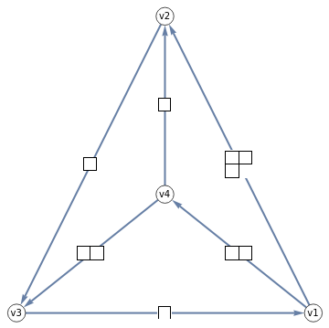
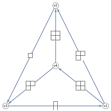
TetGraph[{{j1_,j2_,j3_},{l1_,l2_,l3_}}]:=BirdTrackOfWignerCoefficient[{l2,j3,j1,j2,l3,l1},{"v1","v2","v3","v4"}]
Evaluate a tetrahedral spin network covered by six representations of SU(N) expressed as Dynkin labels
In[]:=
SixJColorSymbol[{{j1_,j2_,j3_},{l1_,l2_,l3_}}]:=Wigner6jCoefficient[{l2,j3,j1,j2,l3,l1},{"v1","v2","v3","v4"},{1,1,1,1}]
Translate a Dynkin label to a Young Partition (the number of boxes at each successive row of the Young tableau)
(also implement the reverse operation, even if we may not use it)
(also implement the reverse operation, even if we may not use it)
In[]:=
(*DynkinLabel[youngPartition_]:=Table[Total@youngPartition[[i;;-1]],{i,Length@youngPartition}]*)YoungPartition[dynkinLabel_]:=Table[Total@dynkinLabel[[i;;-1]],{i,Length@dynkinLabel}]//DeleteCases[#,0]&
Draw a Young Diagram
In[]:=
YoungDiagram[dynkinLabel_]:=Module[{youngPartition=YoungPartition@dynkinLabel},If[youngPartition=={0}||youngPartition=={},Graphics[Text[Style["∅",FontSize->16]],ImageSize->16],Graphics[{White,EdgeForm[Thin],Table[Rectangle[{i,-j},{i+1,-(j+1)}],{i,Length[youngPartition]},{j,youngPartition[[i]]}]},ImageSize->16*Length[youngPartition]]]]
The six-j symbol is displayed as a matrix enclosed in curly brackets
In[]:=
SixJForm[m_]:=StyleBox[RowBox[{"{",GridBox[m],"}"}],SpanMaxSize->∞]//DisplayFormSixJForm[{j1_,j2_,j3_,j4_,j5_,j6_}]:=SixJForm[{{j1,j2,j3},{j4,j5,j6}}]
An alternative Row format, without commas, and fixed width a width of 4
In[]:=
Row4[l_]:=Partition[l,4]//Grid
Check some values from the table 4, "6j symbols of SU3", from Bickerstaff et al. (1982)
In[]:=
allowedReps={l221,l0,l1,l11,l2,l22,l21,l3,l33,l31,l32,l42}={{0,1,1},{0,0},{1,0},{0,1},{2,0},{0,2},{1,1},{3,0},{0,3},{2,1},{1,2},{2,2}};dynkinLabels=Association[Thread@Rule[{"0","1","3","3bar","6","6bar","8","10","10bar","15","15bar","27"},allowedReps]]
Out[]=
0{0,1,1},1{0,0},3{1,0},3bar{0,1},6{2,0},6bar{0,2},8{1,1},10{3,0},10bar{0,3},15{2,1},15bar{1,2},27{2,2}
In[]:=
(*DynkinlabelsforA2=SU3,expressedasYoungPartition*)(**l0={0,0};l11={0,1};l1={1,0};l2={2,0};l22={0,2};l21={1,1};**)someSU3SixJ={{{{l0,l0,l0},{l0,l0,l0}},1},{{{l1,l1,l1},{l11,l1,l0}},-1/3},{{{l1,l1,l1},{l11,l1,l0}},-1/3},{{{l21,l11,l1},{l11,l1,l1}},+1/(23)},{{{l21,l2,l1},{l21,l21,l21}},-1/8},{{{l21,l2,l1},{l21,l2,l11}},1/8},{{{l21,l22,l2},{l21,l1,l22}},-1/8},{{{l21,l22,l2},{l21,l22,l1}},-1/8},{}};
Show a grid of BirdTrack graphs of the tetrahedral spin networks and their SU(3) Six-j symbols, with young diagram labelling of representations
In[]:=
Labeled[TetGraph[Map[YoungDiagram,First@#,{2}]],Row[{SixJForm[Map[YoungDiagram,#[[1]],{2}]],," = ",#[[2]]}]]&/@someSU3SixJ[[1;;-2]]//Row4
Out[]=
|
|
|
| ||||||||||||||||||||||||||||||||
|
|
|
|


We extract the allowed reps of SU(N) for a generalized quark colour theory, keeping only the one which have well known members in the case SU(3), and compute their dimension as a polynomial in N
In[]:=
reps=SortBy[Select[AllowedRepresentations,StringTake[#,1]≠"c"&&StringTake[#,-1]!="r"&],(Dim@#/.Nc->3)&];repsdims=((Dim/@reps/.Nc->n)//Simplify);
In[]:=
reps
Out[]=
{0,1,3,6,8,10,15,24,27,35,64}
Foe each of these representations, ordered from left to right by increasing dimension of the instance for SU(3), and from top to bottom by increasing N, we compute the dimension,
In[]:=
Table[repsdims,{n,1,6}]//MatrixForm
Out[]//MatrixForm=
-1 | 1 | 1 | 1 | 0 | 0 | 0 | 0 | 0 | 0 | 0 |
-3 | 1 | 2 | 3 | 3 | 0 | 4 | 5 | 5 | 0 | 7 |
0 | 1 | 3 | 6 | 8 | 10 | 15 | 24 | 27 | 35 | 64 |
20 | 1 | 4 | 10 | 15 | 45 | 36 | 70 | 84 | 256 | 300 |
75 | 1 | 5 | 15 | 24 | 126 | 70 | 160 | 200 | 1050 | 1000 |
189 | 1 | 6 | 21 | 35 | 280 | 120 | 315 | 405 | 3200 | 2695 |
We display this information on a logarithmic plot, and index the curves by the dimension in SU(3), characterizing its shape in SU(n), and provide the polynomial formula for any n
In[]:=
Labeled[ListLogPlot[Table[repsdims,{n,1,6}]//Transpose,Joined->True,PlotLabels->Thread@Rule[repsdims/.n->3,repsdims],ImageSize->Large,Ticks{Table[{n,"SU"<>ToString@n,1},{n,1,6}],Table[{10^k,10^k,1},{k,0,4}]},PlotRange->{{1,6},{1,10000}},PlotRangeClippingTrue],"Dimensions of the quark/gluon representations of SU(n)"]
Out[]=
 |
Dimensions of the quark/gluon representations of SU(n) |
In[]:=
2. Get a list of valid Six-j Symbols for SU(N)
2. Get a list of valid Six-j Symbols for SU(N)
We restrict our choice to particles, excluding bar-type representations
In[]:=
repsRestricted=reps[[1;;9]]
Out[]=
{0,1,3,6,8,10,15,24,27}
We will use some brute-force research now, so we also compute the time (and should pay attention to the memory size)
In[]:=
((RepsSixTuples9=Tuples[repsRestricted,6])//Length)//AbsoluteTiming
Out[]=
{0.034348,531441}
In[]:=
AbsoluteTiming[(ValidRepsSixTuples9=Select[Range[1,Length@RepsSixTuples9],Length@Wigner6jCoefficient[RepsSixTuples9[[#]],{1,1,1,1},{1,1,1,1}]>0&])//Length]
Out[]=
{125.726,660}
In[]:=
(**SixJForm/@RepsSixTuples9[[ValidRepsSixTuples9[[1;;100]]]]Wigner6jCoefficient[#,{1,1,1,1},{1,1,1,1}]&/@RepsSixTuples9[[ValidRepsSixTuples9[[1;;100]]]]/.Nc->n**)
Create the dataset of all SixJSymbols, sorted by value (where the value is the square root of a rational fraction in n )
We display the number of symbols for any given value, and by clicking on it, can access to the list
We display the number of symbols for any given value, and by clicking on it, can access to the list
In[]:=
SixJDataset=Dataset[grouped6j=GroupBy[{SixJForm@#,Wigner6jCoefficient[#,{1,1,1,1},{1,1,1,1}]/.Nc->n}&/@RepsSixTuples9[[ValidRepsSixTuples9[[1;;-1]]]],Last->First]]
Out[]=
| |||||||||||||||||||||||||||||||||||||||||||
We display for each possible value, the first SixJ Symbol attached
In[]:=
SixJDataset[All,1]
Out[]=
| |||||||||||||||||||||||||||||||||||||||||||||||||||||||||||||||||||||||||||||||||||||||||||||||||||||||||||||||||||||||||||||||||||||||||||||||||||||||||||||||||||
In[]:=
Some more analysis of the SU(n) Six-J symbols...
Some more analysis of the SU(n) Six-J symbols...
In[]:=
3. Reduce a non-trivalent spin network to a trivalent spin network
3. Reduce a non-trivalent spin network to a trivalent spin network
In[]:=
Algorithm
Algorithm
Some utility function to work with directed and undirected graphs. The graph should be directed as a spin network, but undirected as a loop bundle.
In[]:=
undirect[directedEdges_]:=UndirectedEdge[First@#,Last@#]&/@directedEdgesdirect[undirectedEdges_]:=DirectedEdge[First@#,Last@#]&/@undirectedEdgespair[directedEdges_]:=List[First@#,Last@#]&/@directedEdges
In[]:=
RulePlot[ResourceFunction["WolframModel"][{{x,y},{x,z}}{{x,y},{x,w},{y,w},{z,w}}]]
Out[]=

evolutionObject = ResourceFunction["WolframModel"][{{x, y}, {x, z}} -> {{x, y}, {x, w}, {y, w}, {z, w}},
{{0, 0}, {0, 0}},
3]
{{0, 0}, {0, 0}},
3]
" Building an evolving graph from WolframModel suitable to decoration by a trivalent spin network";
Define a default size, and the reduction rules which insert a vertex whenever there is a four valent node
In[]:=
graphImSize=400;
In[]:=
TrivalentReductionRules[]:={{{t,x},{t,y},{t,z},{t,w}}{{t,x},{t,y},{t,u},{u,z},{u,w}},(*4valent4incoming*){{x,t},{t,y},{t,z},{t,w}}{{x,t},{t,y},{t,u},{u,z},{u,w}},(*4valent1in3out*){{x,t},{y,t},{t,z},{t,w}}{{x,t},{y,t},{t,u},{u,z},{u,w}},(*4valent2in2out*)(*{{t,x},{t,y},{t,z},{t,w}}{{t,x},{t,y},{u,t},{u,z},{u,w}},*){{x,t},{y,t},{t,z},{t,w},{t,v}}{{x,t},{y,t},{t,u},{u,z},{u,w},{u,v}}(*5valent2in3out*)};
In[]:=
TrivalentReductionRulesFromTetra[]:={{{t,x},{t,y},{t,z},{t,w}}{{t,x},{t,y},{t,u},{u,z},{u,w}},(*4valent4incoming*){{x,t},{t,y},{t,z},{t,w}}{{x,t},{t,y},{t,u},{u,z},{u,w}},(*4valent1in3out*){{x,t},{y,t},{t,z},{t,w}}{{x,t},{y,t},{t,u},{u,z},{u,w}},(*4valent2in2out*)(*{{t,x},{t,y},{t,z},{t,w}}{{t,x},{t,y},{u,t},{u,z},{u,w}},*){{x,t},{y,t},{z,t},{t,w}}{{x,t},{y,t},{t,u},{z,u},{u,w}},(*4valent3in1out*){{x,t},{y,t},{z,t},{w,t}}{{x,t},{y,t},{t,u},{z,u},{w,u}}(*4valent0in4out*)(*{{x,t},{y,t},{t,z},{t,w},{t,v}}{{x,t},{y,t},{t,u},{u,z},{u,w},{u,v}}*)(*5valent2in3out*)};(*RulePlot[ResourceFunction["WolframModel"][#]]&/@TrivalentReductionRules[]//Column*)RulePlot[ResourceFunction["WolframModel"][TrivalentReductionRulesFromTetra[]]]
Out[]=

Grow a WolframModel evolution rule and then reduce it by applying the Trivalent reduction rule
In[]:=
Clear@TrivalentReduce
In[]:=
An utility function to reduce the size of some graphs
In[]:=
ImageRow[l_]:=Image[#,ImageSize->Medium]&/@l//Row
In[]:=
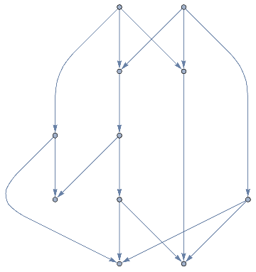
Valence[directedEdges_]:=Max@Tally[Flatten@pair@directedEdges][[All,2]]TrivalentReduce[directedEdges_,level_:0]:=ResourceFunction["WolframModel"][(*TrivalentReductionRules[]*)TrivalentReductionRulesFromTetra[],directedEdges,If[level==0,(Valence[#]-2)&@directedEdges,level]]["FinalState"]SimpleReduce[directedEdges_]:=Union[Select[directedEdges,First@#!=Last@#&]]WolframTrivalentModel[rules_,init_,end_]:=TrivalentReduce[SimpleReduce@ResourceFunction["WolframModel"][rules,init,end]["FinalState"]]WolframTrivalentGraph[rules_,init_,end_]:=Graph[Thread@Rule@@@WolframTrivalentModel[rules,init,end]]
In[]:=
(TrivalentSpinNetworkEvolution=Table[With[{rules={{x,y},{x,z}}{{x,y},{x,w},{y,w},{z,w}},init={{0,0},{0,0}},end=e},WolframTrivalentGraph[rules,init,end]],{e,3,12}])//ImageRow
Out[]=


In[]:=
evolutionObject=ResourceFunction["WolframModel"][{{x,y},{x,z}}{{x,y},{x,w},{y,w},{z,w}},{{0,0},{0,0}},3]fs=evolutionObject["FinalState"](*computefinalstateoftheevolution*)fsnl=Select[fs,First@#!=Last@#&](*removeself-loops*)fsnlu=fsnl//Union(*removehigherlinks*)fsr=First@#->Last@#&/@fs(*buildrules*)fsnlr=First@#->Last@#&/@fsnl(*rulesaftersel-loopsremoval*)fsnlur=First@#->Last@#&/@fsnlu(*rulesafterhigherlinkmerging*)
Out[]=
WolframModelEvolutionObject
|
Out[]=
{{0,3},{1,3},{0,0},{0,4},{0,4},{2,4},{0,2},{0,5},{2,5},{1,5},{1,2},{1,6},{2,6},{3,6}}
Out[]=
{{0,3},{1,3},{0,4},{0,4},{2,4},{0,2},{0,5},{2,5},{1,5},{1,2},{1,6},{2,6},{3,6}}
Out[]=
{{0,2},{0,3},{0,4},{0,5},{1,2},{1,3},{1,5},{1,6},{2,4},{2,5},{2,6},{3,6}}
Out[]=
{03,13,00,04,04,24,02,05,25,15,12,16,26,36}
Out[]=
{03,13,04,04,24,02,05,25,15,12,16,26,36}
Out[]=
{02,03,04,05,12,13,15,16,24,25,26,36}
In[]:=
graphImSize=400;
In[]:=
trivalentObject2=ResourceFunction["WolframModel"][{{{t,x},{t,y},{t,z},{t,w}}{{t,x},{t,y},{t,u},{u,z},{u,w}},(*4valent4incoming*){{x,t},{t,y},{t,z},{t,w}}{{x,t},{t,y},{t,u},{u,z},{u,w}},(*4valent1in3out*){{x,t},{y,t},{t,z},{t,w}}{{x,t},{y,t},{t,u},{u,z},{u,w}},(*4valent2in2out*){{t,x},{t,y},{t,z},{t,w}}{{t,x},{t,y},{u,t},{u,z},{u,w}},{{x,t},{y,t},{t,z},{t,w},{t,v}}{{x,t},{y,t},{t,u},{u,z},{u,w},{u,v}}(*5valent2in3out*)},fsnlu,3]fsnlut=trivalentObject2["FinalState"]fsnlutr=First@#->Last@#&/@fsnlut{Labeled[Graph[fsr,ImageSize->graphImSize],"Graph from WolframModel"],Labeled[Graph[fsnlr,ImageSize->graphImSize],"Reflective edges are removed"],Labeled[Graph[fsnlur,ImageSize->graphImSize],"Multiple edges are merged"],Labeled[Graph[fsnlutr,ImageSize->graphImSize],"Tetravalent nodes are reduced"]}//Row
Out[]=
WolframModelEvolutionObject
|
Out[]=
{{3,6},{0,3},{0,7},{7,4},{7,5},{1,3},{1,8},{8,5},{8,6},{9,5},{9,6},{1,2},{0,2},{2,10},{10,4},{10,9}}
Out[]=
{36,03,07,74,75,13,18,85,86,95,96,12,02,210,104,109}
Out[]=
 |
Graph from WolframModel |
 |
Reflective edges are removed |
 |
Multiple edges are merged |
 |
Tetravalent nodes are reduced |
"The figure below shows the reduction rules we apply to 4-valent or 5-valent nodes";
In[]:=
TrivalentReductionRules[]:={{{t,x},{t,y},{t,z},{t,w}}{{t,x},{t,y},{t,u},{u,z},{u,w}},(*4valent4incoming*){{x,t},{t,y},{t,z},{t,w}}{{x,t},{t,y},{t,u},{u,z},{u,w}},(*4valent1in3out*){{x,t},{y,t},{t,z},{t,w}}{{x,t},{y,t},{t,u},{u,z},{u,w}},(*4valent2in2out*)(*{{t,x},{t,y},{t,z},{t,w}}{{t,x},{t,y},{u,t},{u,z},{u,w}},*){{x,t},{y,t},{t,z},{t,w},{t,v}}{{x,t},{y,t},{t,u},{u,z},{u,w},{u,v}}(*5valent2in3out*)};(*RulePlot[ResourceFunction["WolframModel"][#]]&/@TrivalentReductionRules[]//Column*)RulePlot[ResourceFunction["WolframModel"][TrivalentReductionRules[]]]
Out[]=

"The figure below shows the reduction rules we apply to every possible 4-valent node";
In[]:=
"We could also apply the reduction by a Multiway approach using Multiway rules";
In[]:=
TrivalentMultiwayReductionRules[]:={(*{{t,x},{t,y},{t,z},{t,w}}{{{t,x},{t,y},{t,u},{u,z},{u,w}},{{t,x},{t,z},{t,u},{u,y},{u,w}}}(*4valent4incoming*)*){{{t,x},{t,y},{t,z},{t,w}}{{t,x},{t,y},{t,u},{u,z},{u,w}},{{t,x},{t,y},{t,z},{t,w}}{{t,x},{t,z},{t,u},{u,y},{u,w}}}(*4valent4incoming*)(*{{x,t},{t,y},{t,z},{t,w}}{{x,t},{t,y},{t,u},{u,z},{u,w}},(*4valent1in3out*){{x,t},{y,t},{t,z},{t,w}}{{x,t},{y,t},{t,u},{u,z},{u,w}},(*4valent2in2out*)(*{{t,x},{t,y},{t,z},{t,w}}{{t,x},{t,y},{u,t},{u,z},{u,w}},*){{x,t},{y,t},{t,z},{t,w},{t,v}}{{x,t},{y,t},{t,u},{u,z},{u,w},{u,v}}(*5valent2in3out*)*)};RulePlot[ResourceFunction["WolframModel"][#]]&/@TrivalentMultiwayReductionRules[]//Row
Out[]=

"The figure below shows the longest unoriented cycle on an oriented graph with edges colored upon their codirection (parallel/antiparralel) between graph and cycle";
In[]:=
wt4=TrivalentSpinNetworkEvolution[[2]];wt4vx=wt4//VertexList;wt4undirected=(wt4//EdgeList//undirect//Graph[wt4vx,#]&);wt4cycle=direct/@(%//FindCycle);maxitems=2000;wt4cycles=Table[FindCycle[wt4undirected,{cyclelength},maxitems],{cyclelength,3,Length@First@wt4cycle}];wt4allcycles=FindCycle[wt4undirected,Infinity,All];high=Select[wt4//EdgeList,MemberQ[wt4cycle[[1]],#]&];low=Select[wt4//EdgeList,MemberQ[wt4cycle[[1]],Reverse@#]&];Length/@{wt4cycle[[1]],high,low};Graph[wt4vx,wt4//EdgeList,GraphHighlight->{high,low}];HighlightGraph[Graph[wt4vx,wt4//EdgeList],{Style[#,Red,Thick]&/@high,Style[#,Orange,Thick]&/@low}]
Out[]=

SU(N) is of rank (N-1). We will model a spin network of SU(N) by a covering with loop linear combinations of (N-1) 'colors'.
Our current analysis of how the higher rank intertwiner are build recursively from lower rank intertwiners show that the multi color coverings are not independent but show an emergence. We conjecture a general process and will check it for SU(3) emerging from SU(2). Note that it is also possible to embed the intertwiners down to orthogonal Lie groups instead of unitary. A lot of math there to explore but we try to head directly to some computable results pioneering for the general process.
With this approach we prove a possible way to evaluate spin network on mixed Lie groups, and will give example mixing SU(2) and SU(3).
In[]:=
4. Reduce a trivalent spin network to a sum of product of Wigner Six-j coefficients
4. Reduce a trivalent spin network to a sum of product of Wigner Six-j coefficients
In[]:=
5. Evaluate a trivalent spin network using Penrose/Kauffman/Foxon strand reduction
5. Evaluate a trivalent spin network using Penrose/Kauffman/Foxon strand reduction
In[]:=
Strand Network evaluation (Penrose 1971, Foxon 1994)
Strand Network evaluation (Penrose 1971, Foxon 1994)
Penrose showed how to evaluate a spin network by using the binor calculus [Penrose 1972]. In this approach, a strand network is associated with each spin network by replacing each edge, labelled by spin j, by a linear combination of 2j strands, and summing over all ways of joining these strands at each vertex. So, a vertex is replaced in the strand picture by (3.3) (3.3)
(3.3)  (3.4)where each bar represents an anti-symmetrizer, given by the linear combination of the different ways the 2j strands may cross, with a coefficient of (−1) for each crossing, e.g (3.4)An oriented abstract spin network (where the orientation may be given by the embedding of the spin network in the plane) is evaluated by decomposing each strand network into a number of closed loops using the two basic binor identities [Penrose 1971, 1972],(3.5), (3.6)
 (3.5)
(3.5)  (3.6)These identities form the basis of a topologically invariant diagrammatic calculus[Kauffman 1990], based on the SU(2) invariant tensor εAB represented by (3.7), where additional weights are added, functions of the quantum numbers [n] = Sin(n π/r)/Sin(π/r) such that [r-1]=0, A=^( π /(2 r)).The formulas for dimensions and 6j amplitudes are naturally extended, even for SU(n) to quantum numbers in SU(n)r, where the computation has a cut-off in complexity.
We have explored what the strand approach could be for SU(n) but not found a satisfactory answer in the available time for the project.
Instead we have to use the graph reduction to tetrahedrons and 6j-symbols.
We explored to connect the strands to boxes of the Young tableaux, and make different strand bundles for each rows, copying the nested structure of the SU(n-1) subalgebra of SU(n). More time is needed to confirm that this approach can work and give the same results than the 6j-symbol decomposition.
In[]:=
6. Decorate a trivalent directed graph with representations on edges to create a valid trivalent spin network
6. Decorate a trivalent directed graph with representations on edges to create a valid trivalent spin network
In[]:=
implement the linear solution of cycle covering
implement the linear solution of cycle covering
1) we compute a cycles basis, where each cycle is a set of edges. There is nc cycles and ne edges.
2) each cycle has a value in ^ne ={0,1}^ne, represented by a ne-dimensional vector on the binor field;
all are represented as an nc*ne matrix M over {0,1} with nc rows of ne columns
3) each cycle coloring get a nc-dimensional vectorial value C over ^nc and M.C=L is the label covering of the spin network, a ne-dim vector on
4) a spin network represented by its ne-dim vector L is valid if and only if the system M.C=L is solvable
5) a minimal non trivial valid spin network for a given graph characterized by its matrix M, is a valid L=M.C with all labels>0 and smaller than the smallest constant m>0 for the matrix M.
6) all points before don't depend on the valence of the graph
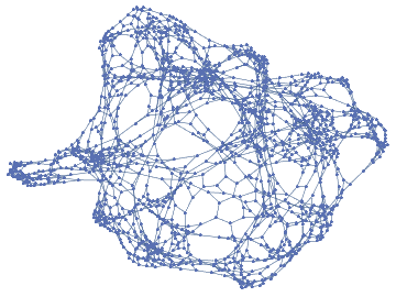
We create a branchial graph from Marcelo Amaral projects, using the Fibonacci rule.
We can setup here the level for the final state, which will have a number of vertices
We can setup here the level for the final state, which will have a number of vertices
In[]:=
rule={"A"->"AB","B"->"A"};initialCondition="A";levelBranchial=6(*20*)(*5*);
In[]:=
Echo[Fibonacci[levelBranchial+1],"Expected number of vertices in the branchial graph : "];
»
Expected number of vertices in the branchial graph : 13
The following function extract the weights on the edges of the causal graph
In[]:=
BranchialEdgeLabelFromCausalGraph[gbranchial_,gcausal_]:=Module[{vertexLabelSpinsAll={},vertexEdges,vertexCausalIncidentsCentral,vertexCausalIncidentsAdjacents,vertexLabelSpins},Do[vertexEdges=AdjacencyList[gbranchial,VertexList[gbranchial][[n]]];(*lookcausalgraphtogetthespinlabeldefinedasthenumberofancestorsincommon(firstlayer)betweenthetwovertices*)vertexCausalIncidentsCentral=AdjacencyList[gcausal,VertexList[gbranchial][[n]]];vertexCausalIncidentsAdjacents=Table[AdjacencyList[gcausal,vertexEdges[[i]]],{i,1,Length[vertexEdges]}];vertexLabelSpins=Table[Length[Intersection[vertexCausalIncidentsCentral,vertexCausalIncidentsAdjacents[[j]]]],{j,1,Length[vertexCausalIncidentsAdjacents]}];vertexLabelSpinsAll=AppendTo[vertexLabelSpinsAll,vertexLabelSpins];,{n,1,VertexCount[gbranchial]}];Return[vertexLabelSpinsAll];]
An utility function to reduce the size of some graphs
In[]:=
ImageRow[l_]:=Image[#,ImageSize->Medium]&/@l//Rowgcausal=ResourceFunction["MultiwaySystem"][rule,initialCondition,levelBranchial,"StatesGraph"], gbranchialgraph=ResourceFunction["MultiwaySystem"][rule,initialCondition,levelBranchial,"BranchialGraph"]//ImageRow
Out[]=
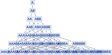

If we look at the final state in the causal graph (the bottom line)
only the leftmost AAA and the rightmost ABBBB don't have a common first level ancestor (one from AAB,ABA,ABBB the "IncidentsCentral")
therefore they don't have a direct link in the branchial graph, meaning they are not siblings
Note that in this genealogic metaphor everyone can have many parents, each parenting by cloning with rule based irradiation
And parents are potential not effective; they could be quantum in the quantum version
In[]:=
gbranchial=ResourceFunction["MultiwaySystem"][rule,initialCondition,levelBranchial,"BranchialGraphStructure"];branchialSpinLabels=BranchialEdgeLabelFromCausalGraph[gbranchial,gcausal];
We build the spin network, undirected, but weighted, and consider that the weights on the edges, either 1 or 2, are spins representations of SO(3)
In[]:=
(*initializationforthelinearoptimization*)fx2[v_,vl_,wl_]:=Thread[First@#->Last@#]&@{UndirectedEdge@@Sort[{v,#}]&/@vl,wl}weightedGraph=Union@Flatten[fx2@@#&/@(Thread[List[VertexList[gbranchial],AdjacencyList[gbranchial,#]&/@VertexList[gbranchial],branchialSpinLabels]])];spingraph=Graph@Flatten[Table[First@#,Last@#]&/@weightedGraph]gcycles=FindCycle[spingraph,{3,Infinity},All];
Out[]=

In[]:=
Echo[gcycles//Length,"Number of cycles nc, equal to the dimension of cycle vector : "];Echo[weightedGraph//Length,"Number of edges ne, equal to the dimension of label vector : "];Echo[Last/@weightedGraph,"Label vector of the proposed spin network : "];orderedEdgeIndices=Association[Thread[First/@weightedGraph->Range@Length@weightedGraph]];reversedEdgeIndices=Association[Thread[Reverse/@First/@weightedGraph->Range@Length@weightedGraph]];edgeIndices=Merge[{orderedEdgeIndices,reversedEdgeIndices},Min]
»
Number of cycles nc, equal to the dimension of cycle vector : 9981373
»
Number of edges ne, equal to the dimension of label vector : 55
»
Label vector of the proposed spin network : {1,2,1,2,2,1,2,1,1,2,1,2,1,2,1,2,1,1,1,1,1,1,2,1,1,1,1,2,1,1,1,1,2,1,2,2,1,1,2,1,1,1,2,1,1,1,1,2,1,2,1,1,2,1,1}
Out[]=
AAAAAAABB1,AAAAAABAB2,AAAAAABBA3,AAAAABAAB4,AAAAABABA5,AAAAABBAA6,AAABBAABAB7,AAABBAABBA8,AAABBAABBBB9,AAABBABAAB10,AAABBABABA11,AAABBABABBB12,AAABBABBABB13,AABABAABBA14,AABABAABBBB15,AABABABAAB16,AABABABABA17,AABABABABBB18,AABABABBAA19,AABABABBABB20,AABABABBBAB21,AABBAAABBBB22,AABBAABABA23,AABBAABABBB24,AABBAABBAA25,AABBAABBBAB26,AABBAABBBBA27,AABBBBABABBB28,AABBBBABBABB29,AABBBBABBBAB30,AABBBBABBBBA31,AABBBBABBBBBB32,ABAABABABA33,ABAABABABBB34,ABAABABBAA35,ABAABABBABB36,ABAABABBBAB37,ABABAABABBB38,ABABAABBAA39,ABABAABBABB40,ABABAABBBAB41,ABABAABBBBA42,ABABBBABBABB43,ABABBBABBBAB44,ABABBBABBBBA45,ABABBBABBBBBB46,ABBAAABBABB47,ABBAAABBBAB48,ABBAAABBBBA49,ABBABBABBBAB50,ABBABBABBBBA51,ABBABBABBBBBB52,ABBBABABBBBA53,ABBBABABBBBBB54,ABBBBAABBBBBB55,AAABBAAAA1,AABABAAAA2,AABBAAAAA3,ABAABAAAA4,ABABAAAAA5,ABBAAAAAA6,AABABAAABB7,AABBAAAABB8,AABBBBAAABB9,ABAABAAABB10,ABABAAAABB11,ABABBBAAABB12,ABBABBAAABB13,AABBAAABAB14,AABBBBAABAB15,ABAABAABAB16,ABABAAABAB17,ABABBBAABAB18,ABBAAAABAB19,ABBABBAABAB20,ABBBABAABAB21,AABBBBAABBA22,ABABAAABBA23,ABABBBAABBA24,ABBAAAABBA25,ABBBABAABBA26,ABBBBAAABBA27,ABABBBAABBBB28,ABBABBAABBBB29,ABBBABAABBBB30,ABBBBAAABBBB31,ABBBBBBAABBBB32,ABABAABAAB33,ABABBBABAAB34,ABBAAABAAB35,ABBABBABAAB36,ABBBABABAAB37,ABABBBABABA38,ABBAAABABA39,ABBABBABABA40,ABBBABABABA41,ABBBBAABABA42,ABBABBABABBB43,ABBBABABABBB44,ABBBBAABABBB45,ABBBBBBABABBB46,ABBABBABBAA47,ABBBABABBAA48,ABBBBAABBAA49,ABBBABABBABB50,ABBBBAABBABB51,ABBBBBBABBABB52,ABBBBAABBBAB53,ABBBBBBABBBAB54,ABBBBBBABBBBA55
We see that even if the algorithm is working well, and FindCycle is very fast, this graph of 55 edges has close to 10 million cycles (or loops).
The linear resolution finding all the solutions would be very using a 55 * 10M matrix.
In this case it is at the limit of the non-computable to get all the solutions.
We will find interesting way of getting some solutions. To show that the spin network is valid, we don't need all the solutions.
Moreover, in this very specific case og representations, it is proved that all trivalent vertices with any combination of spins 1 or 2, therefore 2 or 4 strands, satisfies the triangular inequality. Thus all representation coloring are valid, and the problem is solved.
We used this easy to solve problem to illustrate a method which can quickly diverge in processing time in the general case.
In[]:=
gcycles[[-1]]edgeIndices/@%
Out[]=
{AAAAABAAB,ABAABABBBAB,ABBBABABBBBA,ABBBBAABBBBBB,ABBBBBBABABBB,ABABBBAABBBB,AABBBBABBABB,ABBABBABABA,ABABAAABBA,AABBAAAABB,AAABBAABAB,AABABABBAA,ABBAAAAAA}
Out[]=
{4,37,53,55,46,28,29,40,23,8,7,19,6}
In[]:=
Table[{#,i}->1&/@(edgeIndices/@gcycles[[i]]),{i,4}]//Flatten
Out[]=
{{53,1}1,{55,1}1,{54,1}1,{45,2}1,{55,2}1,{46,2}1,{31,3}1,{45,3}1,{28,3}1,{28,4}1,{46,4}1,{32,4}1}
In[]:=
Now we repeat the process with a graph having less cycles, to show the complete resolution of a given attribution of representation to the edges (decorated spin network).
Now we repeat the process with a graph having less cycles, to show the complete resolution of a given attribution of representation to the edges (decorated spin network).
In[]:=
levelBranchial=4(*20*)(*5*);rule={"A"->"AB","B"->"A"};initialCondition="A";Echo[Fibonacci[levelBranchial+1],"Expected number of vertices in the branchial graph : "];gcausal=ResourceFunction["MultiwaySystem"][rule,initialCondition,levelBranchial,"StatesGraph"], gbranchialgraph=ResourceFunction["MultiwaySystem"][rule,initialCondition,levelBranchial,"BranchialGraph"]//ImageRowgbranchial=ResourceFunction["MultiwaySystem"][rule,initialCondition,levelBranchial,"BranchialGraphStructure"];branchialSpinLabels=BranchialEdgeLabelFromCausalGraph[gbranchial,gcausal];weightedGraph=Union@Flatten[fx2@@#&/@(Thread[List[VertexList[gbranchial],AdjacencyList[gbranchial,#]&/@VertexList[gbranchial],branchialSpinLabels]])];spingraph=Graph@Flatten[Table[First@#,Last@#]&/@weightedGraph]gcycles=FindCycle[spingraph,{3,Infinity},All];Echo[gcycles//Length,"Number of cycles nc, equal to the dimension of cycle vector : "];Echo[weightedGraph//Length,"Number of edges ne, equal to the dimension of label vector : "];Echo[Last/@weightedGraph,"Label vector of the proposed spin network : "];orderedEdgeIndices=Association[Thread[First/@weightedGraph->Range@Length@weightedGraph]];reversedEdgeIndices=Association[Thread[Reverse/@First/@weightedGraph->Range@Length@weightedGraph]];edgeIndices=Merge[{orderedEdgeIndices,reversedEdgeIndices},Min]
»
Expected number of vertices in the branchial graph : 5
Out[]=


Out[]=

»
Number of cycles nc, equal to the dimension of cycle vector : 26
»
Number of edges ne, equal to the dimension of label vector : 9
»
Label vector of the proposed spin network : {1,2,1,2,1,1,2,1,1}
Out[]=
AAAAABB1,AAAABAB2,AAAABBA3,AABBABAB4,AABBABBA5,AABBABBBB6,ABABABBA7,ABABABBBB8,ABBAABBBB9,AABBAAA1,ABABAAA2,ABBAAAA3,ABABAABB4,ABBAAABB5,ABBBBAABB6,ABBAABAB7,ABBBBABAB8,ABBBBABBA9
In[]:=
cycleMatrix=SparseArray[Flatten@Table[{#,i}->1&/@(edgeIndices/@gcycles[[i]]),{i,Length@gcycles}]]
Out[]=
SparseArray
|
In[]:=
cut=36;mcut=Min[Length@gcycles,cut];onesol=LinearSolve[cycleMatrix[[All,1;;mcut]]//Normal,3(Last/@weightedGraph)[[1;;-1]]];If[VectorQ[onesol],{onesol//SparseArray,(onesol//SparseArray).Array[cy,{mcut}]}]
Out[]=
SparseArray
,++++3cy[8]+3cy[10]
|
3cy[1]
2
3cy[2]
2
3cy[6]
2
3cy[7]
2
In[]:=
In[]:=
(mymatrix=cycleMatrix[[All,1;;mcut]])//MatrixForm(myvector=2(Last/@weightedGraph)[[1;;-1]])
Out[]//MatrixForm=
0 | 0 | 0 | 0 | 0 | 0 | 0 | 1 | 1 | 0 | 0 | 0 | 0 | 0 | 1 | 1 | 1 | 1 | 0 | 0 | 1 | 1 | 1 | 1 | 0 | 0 |
0 | 0 | 0 | 0 | 0 | 0 | 0 | 1 | 0 | 1 | 0 | 0 | 0 | 0 | 1 | 1 | 0 | 0 | 1 | 1 | 1 | 1 | 0 | 0 | 1 | 1 |
0 | 0 | 0 | 0 | 0 | 0 | 0 | 0 | 1 | 1 | 0 | 0 | 0 | 0 | 0 | 0 | 1 | 1 | 1 | 1 | 0 | 0 | 1 | 1 | 1 | 1 |
0 | 1 | 1 | 0 | 1 | 1 | 0 | 1 | 0 | 0 | 1 | 1 | 1 | 0 | 0 | 0 | 1 | 0 | 1 | 0 | 0 | 0 | 1 | 0 | 1 | 0 |
0 | 1 | 1 | 0 | 1 | 0 | 1 | 0 | 1 | 0 | 1 | 1 | 0 | 1 | 1 | 0 | 0 | 0 | 1 | 0 | 0 | 1 | 0 | 0 | 0 | 1 |
0 | 0 | 0 | 0 | 0 | 1 | 1 | 0 | 0 | 0 | 0 | 0 | 1 | 1 | 0 | 1 | 0 | 1 | 0 | 0 | 1 | 0 | 0 | 1 | 1 | 1 |
1 | 1 | 1 | 1 | 1 | 0 | 0 | 0 | 0 | 1 | 0 | 0 | 1 | 1 | 1 | 0 | 1 | 0 | 0 | 0 | 1 | 0 | 0 | 1 | 0 | 0 |
1 | 0 | 0 | 1 | 0 | 1 | 0 | 0 | 0 | 0 | 1 | 1 | 0 | 1 | 0 | 1 | 0 | 0 | 0 | 1 | 0 | 1 | 1 | 1 | 0 | 1 |
1 | 0 | 0 | 1 | 0 | 0 | 1 | 0 | 0 | 0 | 1 | 1 | 1 | 0 | 0 | 0 | 0 | 1 | 0 | 1 | 1 | 1 | 1 | 0 | 1 | 0 |
Out[]=
{2,4,2,4,2,2,4,2,2}
In[]:=
vectorsol=LinearSolve[mymatrix,myvector]mymatrix.vectorsol==myvector
Out[]=
{1,1,0,0,0,1,1,2,0,2,0,0,0,0,0,0,0,0,0,0,0,0,0,0,0,0}
Out[]=
True
In[]:=
mymatrix//Dimensionsmyvector//Dimensions(cyV2=Array[cy,{mcut}])//Shortvectorsolsc=FindInstance[mymatrix.cyV2==myvector&&cyV2>=0cyV2,cyV2,Integers,200];Length@vectorsolsc(vectorsols=Map[Last,vectorsolsc,{2}])//Transpose//ArrayPlotTotal/@vectorsolsLength@*DeleteCases[0]/@vectorsols
Out[]=
{9,26}
Out[]=
{9}
Out[]//Short=
{cy[1],cy[2],cy[3],cy[4],cy[5],cy[6],cy[7],cy[8],cy[9],9,cy[19],cy[20],cy[21],cy[22],cy[23],cy[24],cy[25],cy[26]}
Out[]=
89
Out[]=

Out[]=
{7,7,7,7,7,7,7,7,7,7,7,7,7,7,7,7,7,7,7,7,8,7,7,7,7,7,7,7,7,7,7,7,7,7,7,7,8,7,7,7,7,7,7,7,7,7,7,7,7,7,7,7,7,7,7,8,7,7,7,7,7,7,7,7,7,7,7,7,7,7,8,7,7,7,7,7,7,8,7,7,7,7,7,7,7,8,7,7,7}
Out[]=
{5,5,6,6,6,6,6,7,6,6,6,6,6,6,7,7,6,6,7,7,6,6,6,6,6,7,6,6,6,7,7,7,6,6,7,7,6,7,6,6,6,6,6,6,7,6,6,6,7,7,7,6,6,7,7,6,7,7,7,7,6,6,6,6,7,7,6,6,7,7,6,6,7,6,6,7,7,6,7,6,7,6,6,7,7,6,7,7,6}
The graph has exactly 89 possible coverings by loops.
In[]:=
We can modify the algorithm to find some solutions instead of all solutions
We can modify the algorithm to find some solutions instead of all solutions
7. Decorate a non-trivalent directed graph with representations on edges to create a valid non-trivalent spin network
7. Decorate a non-trivalent directed graph with representations on edges to create a valid non-trivalent spin network
The following figure illustrates Penrose's method to evaluate strand networks on the simplest non trivial closed strand network on a tetrahedron. A flattened tetrahedron at the left shows how the final number of loops could be 1 or 3. The instantiation of the anti symmetrizers are shown in the right with their number of braiding.
Figure: Penrose algorithm
Figure: Penrose algorithm


Concluding remarks
Concluding remarks
We found a notion of color spin networks with support on evolution history directed graphs. We have used the Wolfram Model to reduce arbitrary valence growing networks to trivalent versions in a consistent way. The Six-j symbol weights for the evaluation are analytical functions of n, the order of the compact Lie group considered, and are decreasing with n. We have implemented an algorithm to solve the loop covering of a strand network using linear solving for small networks. The problem of large n limit is therefore accessible. The computability for large network can be helped by adapting to quantum groups.
Keywords
Keywords
◼
Multiway Systems
◼
Single Evolution History Graphs
◼
Spin Networks
◼
Compact Lie Groups
◼
Charge-Spin Networks
◼
Color Spin Networks
Acknowledgment
Acknowledgment
I acknowledge Marcelo Amaral, which worked in the same project proposal, for many useful discussions, Klee Irwin for the support, Stephen Wolfram and his group for suggesting a project on “Find spin networks consistent with a given directed graph and compact Lie group” and discussions, Xerxes Arsiwalla for discussions and Jon Lederman for discussions and support.
Reference
Reference
◼
1. Ardonne, E. & Slingerland, J.K.Clebsch - Gordan and 6 j - coefficients for rank two quantum groups.Journal of Physics A : Mathematical and Theoretical 43, 395205 (2010).
◼
2. Arnold, P.The LPM effect in sequential bremsstrahlung : from large - N QCD to N = 3 via the SU (N) analog of Wigner 6 - j symbols.Phys.Rev.D 100, 034030 (2019).
◼
3. Bickerstaff, R.P., Butler, P.H., Butts, M.B., Haase, R.W. & Reid, M.F.3 jm and 6 j tables for some bases of SU 6 and SU 3. Journal of Physics A : Mathematical and General 15, 1087–1117 (1982).
◼
4. Chubb, J., Eskandarian, A. & Harizanov, V.Logic and Algebraic Structures in Quantum Computing.356.
◼
5. Cvitanović, P.Group theory : birdtracks, Lie' s, and exceptional groups.(Princeton University Press, 2008).
◼
6. de Swart, J.J.The Octet Model and its Clebsch - Gordan Coefficients.Rev.Mod.Phys.35, 916–939 (1963).
◼
7. Elvang, H.Birdtracks, Young Projections, Colours.(University of Edinburg, 1999).
◼
8. Elvang, H., Cvitanović, P. & Kennedy, A.D.Diagrammatic Young projection operators for U (n).Journal of Mathematical Physics 46, 043501 (2005).
◼
9. Elvang, H. & Huang, Y.Scattering Amplitudes in Gauge Theory and Gravity.(Cambridge University Press, 2015).doi : 10.1017/CBO9781107706620.
◼
10. Finkelstein, R.J.ON q - SU (3) GLOBAL GAUGE THEORY.Int.J.Mod.Phys.A 19, 443–458 (2004).
◼
11. Foxon, T.J.Spin Networks, Turaev - Viro Theory and the Loop Representation.Class.Quantum Grav.12, 951–964 (1995).
◼
12. Horst, C. & Reuter, J.CleGo : A package for automated computation of Clebsch–Gordan coefficients in tensor product representations for Lie algebras A–G.Computer Physics Communications 182, 1543–1565 (2011).
◼
13. Kaeding, T.A.Tables of SU (3) Isoscalar Factors.Atomic Data and Nuclear Data Tables 61, 233–288 (1995).
◼
14. Kaeding, T.A. & Williams, H.T.Program for generating tables of SU (3) coupling coefficients.Comput.Phys.Commun.98, 398–414 (1996).
◼
15. Kauffman, L.Spin networks and the bracket polynomial.Banach Center Publ.42, 187–204 (1998).
◼
16. Kauffman, L.H. & Lomonaco, S.J.Spin Networks, Quantum Topology and Quantum Computation.in Logic, Language, Information and Computation (eds.Leivant, D. & de Queiroz, R.) vol.4576 248–263 (Springer Berlin Heidelberg, 2007).
◼
17. Kauffman, L.H. & Lomonaco, S.J.q - DEFORMED SPIN NETWORKS, KNOT POLYNOMIALS AND ANYONIC TOPOLOGICAL QUANTUM COMPUTATION.J.Knot Theory Ramifications 16, 267–332 (2007).
◼
18. Keppeler, S. & Sjodahl, M.Orthogonal multiplet bases in SU (Nc) color space.J.High Energ.Phys.2012, 124 (2012).
◼
19. Kisielowski, M. & Based on work done in collaboration with prof.Jerzy Lewandowski and Jacek Puchta.Dynamics of Loop Quantum Gravity encoded in graphs.Journal of Physics : Conference Series 360, 012048 (2012).
◼
20. Kuhn, M. & Walliser, H.Program for calculating SU (4) Clebsch–Gordan coefficients.Computer Physics Communications 179, 733–740 (2008).
◼
21. Penrose, R.Angular momentum : an approach to combinatorial spacetime.in Living Reviews in Relativity http : // www.livingreviews.org/lrr - 2008 - 5 Carlo Rovelli (Citeseer, 1971).
◼
22. Prakash, J.S. & Sharatchandra, H.S.A calculus for SU (3) leading to an algebraic formula for the Clebsch–Gordan coefficients.Journal of Mathematical Physics 37, 6530–6569 (1996).
◼
23. Quantum Gravity at CPT Marseille.GFT, tensors, and random geometries - Lecture 1 - Edward Wilson - Ewing.
◼
24. Quantum Gravity at CPT Marseille.GFT, tensors, and random geometries - Lecture 2 - Edward Wilson - Ewing.
◼
25. Rowe, D.J. & Bahri, C.Clebsch–Gordan coefficients of SU (3) in SU (2) and SO (3) bases.Journal of Mathematical Physics 41, 6544–6565 (2000).
◼
26. Sharp, R.T.Simple Derivation of the Clebsch - Gordan Coefficients.American Journal of Physics 28, 116–118 (1960).
◼
27. Sjödahl, M.ColorMath - A package for color summed calculations in SU (Nc).Eur.Phys.J.C 73, 2310 (2013).
◼
28. Sjodahl, M. & Thoren, J.Decomposing color structure into multiplet bases.arXiv : 1507.03814[hep - ph, physics : hep - th] (2015).
◼
29. Sjodahl, M. & Thorén, J.QCD multiplet bases with arbitrary parton ordering.J.High Energ.Phys.2018, 198 (2018).30. Williams, H.T.SU (3) isoscalar factors.J.Math.Phys.37, 4187–4198 (1996).
◼
31. Yutsis, A.P., Levinson, I.B. & Vanagas, V.V.THE THEORY OF ANGULAR MOMENTUM.173.
◼
32. Clebsch–Gordan coefficients for SU (3).Wikipedia (2019).
◼
33. Marcin_Kisielowski _Loops17.pdf.34. SU (N) Clebsch - Gordan coefficients.https : // homepages.physik.uni - muenchen.de/~vondelft/Papers/ClebschGordan /.
◼
34. Amaral, M., Aschheim, R. & Irwin, K. Quantum Gravity at the Fifth Root of Unity, arXiv:1903.10851 [hep-th] (2019).
◼
35. Wolfram S., A Project to Find the Fundamental Theory of Physics. Wolfram Media. (2020).
Cite this as: Raymond ASCHHEIM, "Color Spin Networks" from the Notebook Archive (2021), https://notebookarchive.org/2021-07-60j8gfo
Download
