Hypocycloids: Using Vector Functions (II)
Author
Tomas Garza
Title
Hypocycloids: Using Vector Functions (II)
Description
This notebook introduces slippage in the motion of the rolling circle
Category
Working Material
Keywords
hypocycloids, slippage, roses
URL
http://www.notebookarchive.org/2023-03-6iqj5a2/
DOI
https://notebookarchive.org/2023-03-6iqj5a2
Date Added
2023-03-14
Date Last Modified
2023-03-14
File Size
89.93 kilobytes
Supplements
Rights
CC0 1.0

Hypocycloids: Using Vector Functions (II)
Hypocycloids: Using Vector Functions (II)
Tomas Garza
Description
Description
In a previous notebook [*] we considered the case where a moving circle rolls along the inside of the circumference of a fixed circle (the moving, or rolling, circle is also called generating circle). The curve that describes a point located at the end of a given radius of the rolling circle is called a hypocycloid, and it was studied on the condition that the generating circle rolls without slippage. The results show a behavior of the curve such that peaks or cusps occur at the points of contact with the fixed circle.
We presented a code to produce these curves, and their behavior (basically the number of cusps) depends on he radius of the generating circle. Furthermore, the function stella [cf.] had a restriction on the ratio of the radii of the fixed and the rolling circles, namely that n, (that ratio) should be equal or larger than 3. Why? Well, if n = 1, both circles are equal and nothing happens; and if n = 2, the resulting curve is just a straight line along the diameter of the white circle (try it).
We presented a code to produce these curves, and their behavior (basically the number of cusps) depends on he radius of the generating circle. Furthermore, the function stella [cf.] had a restriction on the ratio of the radii of the fixed and the rolling circles, namely that n, (that ratio) should be equal or larger than 3. Why? Well, if n = 1, both circles are equal and nothing happens; and if n = 2, the resulting curve is just a straight line along the diameter of the white circle (try it).
We now allow the generating circle to slip or “skid” as it rolls.
[*] https://notebookarchive.org/2023-03-622hvfx
A particular case
A particular case
Consider now the case where the radius of the rolling circle is half the radius of the fixed circle. Make a slight change in the code, so that the gray angle, which determines the speed at which the circle rolls, is twice as large as before. Evaluate the following input cell, and watch the result. An interesting phenomenon occurs: the path of the green point has no longer any cusps, and a smooth curve is now described, forming three loops as it rolls. This is called a three-petal rose.
In[]:=
Framed[Column[{Row[{Spacer[25],Style[Grid[{{"Hypocycloid: the green circle rolls, without slippage,"},{"along the inner part of the white circumference, and the"},{"radius of the green one is one-half the radius of the white"}}],"Label",14]}],Panel@Manipulate[Module[{cen={0,0},fixedCircle,centersCircle,yellowPoint,rollingCircle,greenAngle,grayAngle,greenVector,greenPoint,whiteArrow,redArrow,greenArrow},fixedCircle={White,Circle[cen,1]};centersCircle={Opacity[0.8],Yellow,Circle[cen,0.5]};yellowPoint={Yellow,PointSize[0.02],Point[0.5cs[ang]]};rollingCircle={Green,Opacity[0.7],Circle[0.5cs[ang],0.5]};greenAngle={Opacity[0.5],Green,Disk[cen,0.5,{0,ang}]};grayAngle={Opacity[0.7],White,Disk[0.5cs[ang],0.5,{0,-2ang}]};greenVector=-0.5cs[π-2ang]+0.5cs[ang];greenPoint={Green,PointSize[0.02],Point[greenVector]};whiteArrow={White,Arrowheads[0.03],Arrow[{cen,-0.5cs[π-2ang]}]};redArrow={Red,Arrowheads[0.03],Arrow[{cen,0.5cs[ang]}]};greenArrow={Green,Arrowheads[0.03],Arrow[{cen,greenVector}]};ParametricPlot[-0.5cs[π-2t]+0.5cs[t],{t,0.01,ang},PlotStyle{Orange,Thickness[0.006]},Epilog->{Inset[Style[Grid[{{"the green point describes a three-petal rose"}}],14,White],{0,1.4}],Point[cen],greenPoint,yellowPoint,fixedCircle,rollingCircle,Translate[whiteArrow,0.5cs[ang]],If[k>1,{greenAngle,grayAngle,centersCircle,whiteArrow,greenArrow,redArrow,{Red,PointSize[0.02],Point[cen]}}]},Axes->True,TicksNone,Background->Black,PlotRange1.7,ImageSize450]],{{k,1,Grid[{{"1 simple view"},{"2 constructive view"}}]},{1,2}},{{ang,0,"ϕ"},0,2π},Initialization{cs[x_]:={Cos[x],Sin[x]}}]}],RoundingRadius8]
Out[]=
| ||||||||||||||||
| ||||||||||||||||


The non-slippage in the rolling process actually means in this case that the green circle gives two complete turns (watch the process moving the slider: initially, the white arrow is horizontal and, as the circle rolls, it returns to this position when ϕ = π, and again when ϕ = 2π). Its radius is 0.5, so its circumference is π, and two complete turns are equivalent to a total distance of 2π, which is also the length of the white circumference.
Introducing slippage in the process
Introducing slippage in the process
To this effect we change the angle controlling the turning speed of the green circle; i.e. the definition of grayAngle in the code. In the previous example it had a coefficient of 2; and now we write r = +2instead, where dist , the distance from the circumference of the fixed circle to the center of the is taken to be 0.5 (cf. below). In the figure we can observe the effect of this change.
(1-dist)
dist
In[]:=
FramedColumnRow[{Spacer[35],Style[Grid[{{"Hypocycloid: the green circle rolls along the inner part of"},{"the white circumference, allowing for a slight degree of slippage"}}],"Label",14]}],Panel@ManipulateModule{cen={0,0},dist,fac,fixedCircle,centersCircle,yellowPoint,rollingCircle,greenAngle,grayAngle,greenVector,greenPoint,whiteArrow,redArrow,greenArrow},dist=0.5;(*dististhedistancefromthecircumferenceofthefixedcircletothecenteroftherollingcircle*)fac=+2(**);fixedCircle={White,Circle[cen,1]};centersCircle={Opacity[0.8],Yellow,Circle[cen,1-dist]};yellowPoint={Yellow,PointSize[0.02],Point[(1-dist)cs[ang]]};rollingCircle={Green,Opacity[0.7],Circle[(1-dist)cs[ang],dist]};greenAngle={Opacity[0.5],Green,Disk[cen,dist,{0,ang}]};grayAngle={Opacity[0.7],White,Disk[(1-dist)cs[ang],dist,{0,-facang}]};greenVector=-(dist)cs[π-facang]+(1-dist)cs[ang];greenPoint={Green,PointSize[0.02],Point[greenVector]};whiteArrow={White,Arrowheads[0.03],Arrow[{cen,(-dist)cs[π-facang]}]};redArrow={Red,Arrowheads[0.03],Arrow[{cen,(1-dist)cs[ang]}]};greenArrow={Green,Arrowheads[0.03],Arrow[{cen,greenVector}]};ParametricPlot[-(dist)cs[π-fact]+(1-dist)cs[t],{t,0.01,ang},PlotStyle{Orange,Thickness[0.006]},Epilog->{Inset[Style[Grid[{{"the green point describes a rose with four petals"}}],14,White],{0,1.4}],Point[cen],greenPoint,yellowPoint,fixedCircle,rollingCircle,Translate[whiteArrow,(1-dist)cs[ang]],If[k>1,{greenAngle,grayAngle,centersCircle,whiteArrow,greenArrow,redArrow,{Red,PointSize[0.02],Point[cen]}}]},Axes->True,TicksNone,Background->Black,PlotRange1.7,ImageSize450],{{k,1,Grid[{{"1 simple view"},{"2 constructive view"}}]},{1,2}},{{ang,0,"ϕ"},0,2π},Initialization{cs[x_]:={Cos[x],Sin[x]}},RoundingRadius8
(1-dist)
dist
Out[]=
| ||||||||||||||||
| ||||||||||||||||

The radius of the fixed circle is 1 so that its circumference is 2 π, while the radius of the green circle is 0.5, so that its circumference is π, and hence the complete path of the latter would require just two complete turns. However, we can see in the above figure (moving the slider to the far right) that the rolling circle makes three turns, instead of two! This means that some “slippage” occurs along the process, and this is what results in the formation of loops in the curve.
Generating roses with n petals
Generating roses with n petals
As we did in the case of stars, I here propose a function to generate a rose with an integral number of petals (three or more). This function assumes that the the radius of the rolling disk is always half of that of the fixed one. I limit the number to 20, in order to avoid cluttering in the image.
In[]:=
Clear[rosita];rosita[n_?IntegerQ/;3≤n≤20]:=FramedPanel@ManipulateModule{cen={0,0},dist,fac,st,fixedCircle,centersCircle,yellowPoint,rollingCircle,greenAngle,grayAngle,greenVector,greenPoint,whiteArrow,redArrow,greenArrow},dist=0.5(*dististhedistancefromthecircumferenceofthefixedcircletothecenteroftherollingcircle*);fac=+n-2(**);st=ToString[n];fixedCircle={White,Circle[cen,1]};centersCircle={Opacity[0.8],Yellow,Circle[cen,1-dist]};yellowPoint={Yellow,PointSize[0.02],Point[(1-dist)cs[ang]]};rollingCircle={Green,Opacity[0.7],Circle[(1-dist)cs[ang],dist]};greenAngle={Opacity[0.5],Green,Disk[cen,dist,{0,ang}]};grayAngle={Opacity[0.7],White,Disk[(1-dist)cs[ang],dist,{0,-facang}]};greenVector=-(dist)cs[π-facang]+(1-dist)cs[ang];greenPoint={Green,PointSize[0.02],Point[greenVector]};whiteArrow={White,Arrowheads[0.03],Arrow[{cen,(-dist)cs[π-facang]}]};redArrow={Red,Arrowheads[0.03],Arrow[{cen,(1-dist)cs[ang]}]};greenArrow={Green,Arrowheads[0.03],Arrow[{cen,greenVector}]};ParametricPlot[-(dist)cs[π-fact]+(1-dist)cs[t],{t,0.01,ang},PlotStyle{Orange,Thickness[0.006]},Epilog->{Inset[Style[Grid[{{"the green point describes a rose with "<>st<>" petals"}}],14,White],{0,1.4}],Point[cen],greenPoint,yellowPoint,fixedCircle,rollingCircle,Translate[whiteArrow,(1-dist)cs[ang]],If[k>1,{greenAngle,grayAngle,centersCircle,whiteArrow,greenArrow,redArrow,{Red,PointSize[0.02],Point[cen]}}]},Axes->True,TicksNone,Background->Black,PlotRange1.7,ImageSize450],{{k,1,Grid[{{"1 simple view"},{"2 constructive view"}}]},{1,2}},{{ang,0,"ϕ"},0,2π},Initialization{cs[x_]:={Cos[x],Sin[x]}},RoundingRadius->5
(1-dist)
dist
After execution of the above cell, the function rosita[n] generates a rose with n petals. So, for example, for n = 10, we get
In[]:=
rosita[10]
Out[]=
|  | ||||||||||||
|
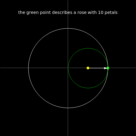
Notice that, in general, the number of complete turns of the rolling circle is one less than the number of petals.
Cite this as: Tomas Garza, "Hypocycloids: Using Vector Functions (II)" from the Notebook Archive (2023), https://notebookarchive.org/2023-03-6iqj5a2
Download
