Educational Materials

Numerical solution of Laplace's equation in finite 2D domains. Application to the analysis of electric potential maps in the Physics lab

E. de Lorenzo Poza, Antonio Badía-Majós

Author

E. de Lorenzo Poza, Antonio Badía-Majós

Title

Numerical solution of Laplace's equation in finite 2D domains. Application to the analysis of electric potential maps in the Physics lab

Description

Notebook for the simulation of electric potential distributions in experimental physics courses

Numerical solution of Laplace’s equation in finite 2D domains
Application to the Analysis of Electric Potential Maps in the Physics Lab
E. de Lorenzo Poza and A. Badía-Majós

Two-dimensional electric potential maps are a valuable tool in physics courses. A simple experiment readily available in a conventional lab allows us to introduce a number of ideas concerning the electric field E and potential Φ. Nevertheless, non-trivial geometries are hardly treated by means of analytical methods and require numerical evaluations in order to get quantitative predictions. We emphasize that with the aid of Mathematica the student may compare the experimental results to theoretical expectations, and obtain a high degree of success. Relying on several built-in functions, one may produce relatively simple notebooks corresponding to various interesting geometries as those presented in this notebook.

Introduction. The physical problem

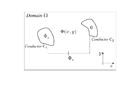
As sketched in the figure below, typically, the 2D mapping problem consists of finding the constant potential lines around a given configuration of conducting electrodes (named

and

) that are embedded in a weakly conducting sheet (domain Ω) and kept at a constant potential difference

by means of a battery. As one may readily find in standard intermediate Electromagnetic courses, theoretically, the electrostatic potential may be calculated by solving Laplace’s equation with the specified (Dirichlet) boundary conditions within the body of the electrodes (i.e.

and

), and Neumann boundary conditions at the boundary of the domain (i.e. ∂ Ω). The latter correspond to the physical condition that the circulating currents may not leave the conducting sheet. Below in this notebook, the statement of Dirichlet boundary conditions may be explicitly observed. Neumann conditions at the region’s boundary do not appear as they are implicitly imposed by Mathematica unless otherwise stated.
In brief, the calculation method will consist of first obtaining the function

(x,y) and eventually using E = -grad

Numerical solution

Mathematica’s built-in functions allow us to easily define the differential equation, the domain, and the boundary conditions of the problem of which we want to find a numerical solution. In that sequence, we may define the differential equation with the function Laplacian, the region of interest may be expressed as a combination of basic regions (Rectangle, Disk,...) through basic set operations (RegionUnion, RegionDifference, RegionIntersection,...) and the boundary conditions, corresponding to the potential at the conductors introduced by DirichletCondition. It is also possible to explicitly state a perpendicularity condition for the potential [

∂

Φ = F(x,y)] with NeumannValue. As it has been mentioned above, the solver assumes null Neumann conditions (

∂

Φ = 0) on the boundary of the domain unless otherwise indicated. In our case this fits the physical condition that electrons must flow along the boundary of the medium (carbon paper) and not across. Then, perpendicularity of equipotentials and electric flow leads to

∂

Φ = 0. The potential is finally calculated using NDSolve and, from that, the electric field may be derived with the built-in function Grad. The results may be visualized as below with ContourPlot and StreamPlot. The usual options for graphics available in Mathematica enable a convenient visual output, as one may readily check. We display equipotentials and electric field lines.
Corresponding to the configurations investigated in our work Eur. J. Phys. 39 065201, below we include the evaluation cells that allow to solve the field/potential problem for the so called monopole and dipole configurations. As shown, they arise when the conductors

and

are shaped as colinear strips with one or two tiny slits in between. One may straightforwardly notice that the arising electric field lines and equipotentials may be identified as “reciprocal” to those of the genuine monopole and dipole, with the point charges at the position of the slit.
Apparently, the notebook may be modified with ease so as to generate potential maps for many other geometrical arrangements of domains and electrodes.

Monopole in a circular domain

Let's solve the potential problem for the case of two long conducting strips along the diameter of a circular domain with a tiny separation in between that coincides with the center of the circle. The slit acts as a pole (source) for equipotentials as seen below

 First, we define the object (laplaceEq) corresponding to Laplace’s

equation

laplaceEq=Laplacianϕ[x,y],{x,y}0;

 Then, we define the weakly conducting domain Ω: circle with the electrodes (bar1 and bar2) substracted

bar1=Rectangle[{-10.1,-0.1},{-0.1,0.1}];bar2=Rectangle[{0.1,-0.1},{10.1,0.1}];Π=RegionDifference[RegionDifference[Disk[{0,0},10],bar1],bar2];p2=Graphics[{Black,Rectangle[{-10.1,-.05},{-0.1,.05}]}];p3=Graphics[{Red,Rectangle[{0.1,-.05},{10.1,.05}]}];

 Next, Dirichlet boundary conditions are imposed on the electrodes

C1=DirichletConditionϕ[x,y]0,(y-0.1∨y0.1∨x-0.1)∧x<0;C2=DirichletConditionϕ[x,y]10,(y-0.1∨y0.1∨x0.1)∧x>0;

 Eventually, Laplace's equation is solved

sol=NDSolve{laplaceEq,C1,C2},ϕ,{x,y}∈Π;

 And one may plot (customized) equipotentials with the help of the function ContourPlot

Off[InterpolatingFunction::dmval]equipotentialsc=ContourPlotEvaluateϕ[x,y]/.sol,{x,y}∈Π,PlotLegendsAutomatic,AspectRatioAutomatic,Contours9,BoundaryStyle->{Thick,Gray},FrameFalse,FrameTicksNone;Show[p2,p3,equipotentialsc,PlotLabelEquipotentials]

 Starting with the potential, we evaluate the electric field vector for the circular geometry Ec, and make a plot of the corresponding lines of force, now with the help of the built-in function StreamPlot

Ec=-GradEvaluateϕ[x,y]/.sol,{x,y};

Off[InterpolatingFunction::dmval]field1p=StreamPlot[Ec,{x,-10,10},{y,-10,10},AspectRatioAutomatic,RegionFunctionFunction[{x,y},{x,y}∈Π],StreamPointsTable[{i,0.12},{i,-9.0,-2,3.0}],FrameTicksNone];field1n=StreamPlot[Ec,{x,-10,10},{y,-10,10},AspectRatioAutomatic,RegionFunctionFunction[{x,y},{x,y}∈Π],StreamPointsTable[{i,-0.12},{i,-9.0,-2,3.0}],FrameTicksNone];Show[p2,p3,field1p,field1n,Graphics[{EdgeForm[{Black}],FaceForm[],Circle[{0,0},10]}],PlotLabelElectricfield]

Monopole in a square domain

Let’s now solve the potential problem for the case of two long strips along the central line of a square domain with a tiny separation in between, that coincides with the center of the square. Again, the slit acts as pole (source) for equipotentials as seen below. However, owing to the conditions at the boundary of the domain (
∂
n
Φ = 0), in this case the radial equipotentials undergo a deformation so as to reach the boundary at right angles

 First, we define the object (laplaceEq) corresponding to Laplace’s equation

laplaceEq=Laplacianϕ[x,y],{x,y}0;

 Then, we define the weakly conducting domain Ω: square with the electrodes (bar1 and bar2) substracted

bar1=Rectangle[{-10.1,-0.1},{-0.1,0.1}];bar2=Rectangle[{0.1,-0.1},{10.1,0.1}];Π=RegionDifference[RegionDifference[Rectangle[{-10.1,-10.1},{10.1,10.1}],bar1],bar2];p2=Graphics[{Black,Rectangle[{-11,-.05},{-0.1,.05}]}];p3=Graphics[{Red,Rectangle[{0.1,-.05},{11,.05}]}];

 Next, Dirichlet boundary conditions are imposed on the electrodes

C1=DirichletConditionϕ[x,y]0,(y-0.1∨y0.1∨x-0.1)∧x<0;C2=DirichletConditionϕ[x,y]10,(y-0.1∨y0.1∨x0.1)∧x>0;

 Eventually, Laplace's equation is solved

sol=NDSolve{laplaceEq,C1,C2},ϕ,{x,y}∈Π;

 And one may plot (customized) equipotentials with the help of the function ContourPlot

Off[InterpolatingFunction::dmval]equipotentialss=ContourPlotEvaluateϕ[x,y]/.sol,{x,y}∈Π,PlotLegendsAutomatic,AspectRatioAutomatic,Contours9,BoundaryStyle->{Thin,Gray},FrameFalse;Show[p2,p3,equipotentialss,PlotLabelEquipotentials]

 Starting with the potential, we evaluate the electric field vector for the square geometry Es, and make a plot of the corresponding lines of force,
now with the help of the built-in function StreamPlot

Es=-GradEvaluateϕ[x,y]/.sol,{x,y};Off[InterpolatingFunction::dmval]field1p=StreamPlot[Es,{x,-10,10},{y,-10,10},AspectRatioAutomatic,RegionFunctionFunction[{x,y},{x,y}∈Π],StreamPointsTable[{i,0.1},{i,-9.2,-2,2}],FrameTicksNone];field1n=StreamPlot[Es,{x,-10,10},{y,-10,10},AspectRatioAutomatic,RegionFunctionFunction[{x,y},{x,y}∈Π],StreamPointsTable[{i,-0.1},{i,-9.2,-2,2}],FrameTicksNone];Show[p2,p3,field1p,field1n,Graphics[{EdgeForm[{Black}],FaceForm[],Rectangle[{-10.1,-10.1},{10.1,10.1}]}],PlotLabelElectricfield]

Dipole in conjoined circular/hollow-rectangular domain

As one may guess from the above, and according to our work Eur. J. Phys. 39 065201, a combination of three linear electrodes with two slits in between may be used to produce dipole-like equipotentials. Below, we provide the Mathematica scripts that may be used to explore this situation. In addition, this examples illustrates the possibility of solving Laplace’s equation in conjoined domains. Thus, here we assume that one of the slits is surrounded by a circular barrier that establishes the (Neumann) boundary condition

∂

Φ = 0, as occurs at the limits of the conducting sheet. Physically, this may be achieved by trimming the domain along such boundary. Mathematically, one just solves the differential equation for each domain, and matches solutions through the Dirichlet conditions at the penetrating electrodes (see below).

 Definition of Laplace's equation, equipotential electrodes (bar1, bar2, bar3) and the regions that will support the full problem (Ω =

⋃

laplaceEq=Laplacian[v[x,y],{x,y}]0;

bar1=Rectangle[{-15.1,-0.1},{-3.1,0.1}];bar2=Rectangle[{3.1,-0.1},{15.1,0.1}];bar3=Rectangle[{-2.9,-0.1},{2.9,0.1}];disc1=Disk[{7,0},5.95];disc2=Disk[{7,0},6.05];circle2=Graphics[{Dashed,Circle[{7,0},6]}];p2=Graphics[{Black,Rectangle[{-15,-.02},{-3.3,.02}]}];p3=Graphics[{Red,Rectangle[{-2.7,-.02},{2.7,.02}]}];p4=Graphics[{Black,Rectangle[{3.3,-.02},{15,.02}]}];Π=RegionDifference[RegionDifference[RegionDifference[Rectangle[{-15,-10},{15,10}],bar1],bar2],bar3];Πc=RegionDifference[Rectangle[{-15,-10},{15,10}],Π];Π1=RegionDifference[Π,disc2];Π2=RegionDifference[disc1,Πc];

 For clarity, we plot the two domains that are eventually merged

GraphicsRow[{RegionPlot[Π1,AspectRatioAutomatic,ImageSize450],RegionPlot[Π2,AspectRatioAutomatic,ImageSize200]}]

ItemAspectRatio::shdw:Symbol ItemAspectRatio appears in multiple contexts {System`,Global`}; definitions in context System` may shadow or be shadowed by other definitions.



 Boundary conditions at the interpenetrating electrodes(Ω =

⋃

C1=DirichletCondition[v[x,y]0,(y-0.1∨y0.1∨x-3.1)∧x<-3];C2=DirichletCondition[v[x,y]0,(y-0.1∨y0.1∨x3.1)∧x>3];C3=DirichletCondition[v[x,y]10,(y-0.1∨y0.1∨x2.9∨x-2.9)∧(x>-3∧x<3)];

 Solution of Laplace's equationat each subdomain:

and

sol1=NDSolve[{laplaceEq,C1,C2,C3},v,{x,y}∈Π1];sol2=NDSolve[{laplaceEq,C2,C3},v,{x,y}∈Π2];

 Definition of graphical objects

forthepotential

graph1=ContourPlot[Evaluate[v[x,y]/.sol1],{x,y}∈Π,PlotLegendsNone,AspectRatioAutomatic,Contours{1,2,4,6,8},ColorFunction(If[#1>1/2,White,White]&),FrameTicksNone,ContourLabelsAll,ContourLabelsText[BackgroundWhite],PlotLabelEquipotentials];graph2=ContourPlot[Evaluate[v[x,y]/.sol2],{x,y}∈Π2,PlotLegendsAutomatic,AspectRatioAutomatic,Contours{1,2,4,6,8},PlotRange{-1,11},ColorFunction->"PearlColors",FrameTicksNone];

 Evaluation of electric field

E1=-Grad[Evaluate[v[x,y]/.sol1],{x,y}];E2=-Grad[Evaluate[v[x,y]/.sol2],{x,y}];

field1p=StreamPlot[E1,{x,-15,15},{y,-10,10},AspectRatioAutomatic,RegionFunctionFunction[{x,y},{x,y}∈Π1],StreamPoints{{-2,0.2},{-4,0.2},{-7.0,0.2},{-10.0,0.2},{-12.0,0.2},{-14.0,0.2},{14.0,0.2}},StreamStyleGreen,FrameTicksNone,PlotLabelElectricfield];field1n=StreamPlot[E1,{x,-15,15},{y,-10,10},AspectRatioAutomatic,RegionFunctionFunction[{x,y},{x,y}∈Π1],StreamPoints{{-2,-0.2},{-4.,-0.2},{-7.0,-0.2},{-10.0,-0.2},{-12.0,-0.2},{-14.0,-0.2},{14.0,-0.2}},StreamStyleGreen,FrameTicksNone];field2n=StreamPlot[E2,{x,-10,10},{y,-5,5},AspectRatioAutomatic,RegionFunctionFunction[{x,y},{x,y}∈Π2],StreamPoints{{4.5,-0.2},{7.0,-0.2},{10.0,-0.2},{12.0,-0.2}},FrameTicksNone];field2p=StreamPlot[E2,{x,-10,10},{y,-5,5},AspectRatioAutomatic,RegionFunctionFunction[{x,y},{x,y}∈Π2],StreamPoints{{4.5,0.2},{7.0,0.2},{10.0,0.2},{12.0,0.2}},FrameTicksNone];

 Final plots: joint potential (discontinuous along the cut line)

Show[graph1,graph2,p2,p3,p4,circle2]

 Final plots: joint electric field (parallel to the cut line)

Show[field1p,field1n,field2p,field2n,field2p,p2,p3,p4]

References
A. Badía Majós and E. de Lorenzo Poza, European Journal of Physics , 39 (2018) 065201.

Cite this as: E. de Lorenzo Poza, Antonio Badía-Majós, "Numerical solution of Laplace's equation in finite 2D domains. Application to the analysis of electric potential maps in the Physics lab" from the Notebook Archive (2018), https://notebookarchive.org/2019-04-b1mo7mo