Pseudospectral Chebyshev method finds approximate solutions of the Mathieu’s equations
Author
Le Anh Nhat
Title
Pseudospectral Chebyshev method finds approximate solutions of the Mathieu’s equations
Description
We used the Chebyshev pseudospectral method (CPM) basing on the Chebyshev-Gauss-Lobatto points to compute the approximate solutions.
Category
Academic Articles & Supplements
Keywords
Mathieu’s equations, pseudospectral method, ODEs, Chebyshev
URL
http://www.notebookarchive.org/2019-11-2d1wasc/
DOI
https://notebookarchive.org/2019-11-2d1wasc
Date Added
2019-11-05
Date Last Modified
2019-11-05
File Size
248.21 kilobytes
Supplements
Rights
Redistribution rights reserved

Information and Telecommunication Technologies and Mathematical Modeling of High-Tech Systems - 2019 (ITTMM 2019)
Chebyshev Pseudospectral Method Finds Approximate Solutions of the Mathieu’s Equations
L.A.
*†
Nhat
* Peoples’ Friendship University of Russia, Moscow, 117198, Russia
Tan Trao University, Tuyen Quang, 22227, Vietnam
†
Email: leanhnhat@mail.ru
Mathieu’s equations are second-order linear ordinary differential equations; they have many applications in the engineering and physical sciences. We shall be considering Mathieu’s equations with two-point boundary value on the range [−1, 1] and the given boundary values. We used the Chebyshev pseudospectral method (CPM) basing on the Chebyshev-Gauss-Lobatto points to compute the approximate solutions. In this study, the computer program was written by language Mathematica version 10.4. We made a comparison between the CPM’s numerical results and the Mathematica’s numerical results, the biggest odds were very small.
Key words and phrases: Mathieu, Mathieu’s equations, pseudospectral method, ODEs, Chebyshev.
1. Introduction
1. Introduction
Mathieu’s equation appears in many problems within theoretical physics. Mathieu functions can be applied to describe standing, traveling, and rotating waves in physical systems [1]. Its properties have been applied in recent years as: vibrations in an elliptic drum, the inverted pendulum, the radio frequency quadrupole, frequency modulation, stability of a floating body, alternating gradient focusing, the Paul trap for charged particles, the mirror trap for neutral particles [2], and the radiative transfer problem [3].
We consider the Mathieu’s differential equation (MDE)
u''(x)+(a-2bcos(2x))u(x)=0,-1≤x≤1,u(-1)=,u(1)=,
α
1
β
1
(
1
)and the Mathieu’s modified differential equation (MmDE)
u''(x)-(a-2bcosh(2x))u(x)=0,-1≤x≤1,u(-1)=,u(1)=,
α
2
β
2
(
2
)where a, b ∈ are variable coefficients.
Several methods have been studied to determine the numerical solutions of Mathieu’s equations. Kirkpatrick E. T. built the tables of values of the modified mathieu functions [4]; Abramov A. A. founded eigenvalues with a given index, the stability of solutions to the difference equations, correct definition and calculation of eigenvalues and Mathieu functions with non-integer numbers, correct definition and calculation of the Mathieu characteristic exponent, and the calculation of values of solutions to the Mathieu equation for large arguments [5]; the harmonic balance method based on the given algebraic function to determine the analytic approximations for the critical values and their corresponding periodic solutions of the Mathieu differential equation [6]; the bisection method computed the eigenvalues of Mathieu’s equation were expanded in trigonometric series [7]; Spectral collocation solutions detemined the accurate computation of a large number of specified eigenvalues and eigenvectors of Mathieu’s system as a multiparameter eigenvalue problem [8]; Samuel A. W. had gathered several analytic approximations for various quantities relating to Mathieu’s equation and compared them to numerical results [9], ...
2. Pseudospectral method using the Chebyshev differentiation matrix
2. Pseudospectral method using the Chebyshev differentiation matrix
Suppose that we have p(x) polynomial degree n, and then we can know about values at the points p(), p(), ..., p() and the first and second derivatives p(x) at the same points in expressing matrix form:
x
0
x
1
x
n
p'( x 0 |
p'( x 1 |
⋮ |
p'( x n |
p( x 0 |
p( x 1 |
⋮ |
p( x n |
p''( x 0 |
p''( x 1 |
⋮ |
p''( x n |
2
D
p( x 0 |
p( x 1 |
⋮ |
p( x n |
(
3
)where is an differentiation matrix [10 – 14].
D=
(1)
d
i,j
(n+1)×(n+1)
A grid function is defined on the Chebyshev-Gauss-Lobatto points such that =cos, . They are the extrema of the –th order in the Chebyshev polynomial (x)=cos(nx). The differential matrix at the quadrature points is given by
p(x)
x={,,...,}
x
0
x
1
x
n
x
k
kπ
n
k=0,1,2,...,n
n
T
n
-1
cos
(1)
d
i,j
(1)
d
0,0
(1)
d
n,n
2+1
2
n
6
(1)
d
i,i
x
i
2(1-)
2
x
i
(1)
d
i,j
c
i
c
j
i+j
(-1)
x
i
x
j
(
4
)where
c
k
|
(
5
)Suppose that the second-order differential equation has form
u''(x)=t(x),u(-1)=α,u(1)=β,
(
6
)and the collocation points } so that .
{
x
i
1=>>...>=-1
x
0
x
1
x
n
We know that
u''(x)=().
n
∑
k=0
2
D
i,k
u
n
x
k
(
7
)Therefore, equation (6) becomes
n
∑
k=0
2
D
i,k
u
n
x
k
x
i
u
n
x
n
u
n
x
0
(
8
)Alternately, we partition the matrix into three matrices:
D
(1)
E
(1) d 1,1 | (1) d 1,2 | ⋯ | (1) d 1,n-1 |
(1) d 2,1 | (1) d 2,2 | ⋯ | (1) d 2,n-1 |
⋮ | ⋮ | ⋱ | ⋮ |
(1) d n-1,1 | (1) d n-1,2 | ⋯ | (1) d n-1,n-1 |
(1)
e
0
(1) d 1,0 |
(1) d 2,0 |
⋮ |
(1) d n-1,0 |
(1)
e
n
(1) d 1,n |
(1) d 2,n |
⋮ |
(1) d n-1,n |
(
9
)Or we can rewrite the same short form
(1)
E
(1)
d
i,j
(1)
e
0
(1)
d
i,0
(1)
e
n
(1)
d
i,n
(
10
)Similarly, we partition the matrix into tree matrices: , and .
2
D
(2)
E
(2)
e
0
(2)
e
n
So the equation (6) can then be written in the form matrix
β+u+α=t,u(-1)=α,u(1)=β,
(2)
e
0
(2)
E
(2)
e
n
(
11
)where u, t denote the vectors
u=
,t=
.
u( x 1 |
u( x 2 |
⋮ |
u( x n-1 |
t( x 1 |
t( x 2 |
⋮ |
t( x n-1 |
3. Aplications
3. Aplications
From section 2, the equation (1) can be written in the matrix form
(+Q)u=-+,u(-1)=,u(1)=,
(2)
E
β
1
(2)
e
0
α
1
(2)
e
n
α
1
β
1
(
12
)where denotes diagonal matrices with elements , in the case the Mathieu’s equation.
Q
(a-2bcos(2))
x
i
i=1,2,...n-1
Similarly, the equation (2) can be written in the matrix form
(-P)u=-+,u(-1)=,u(1)=,
(2)
E
β
2
(2)
e
0
α
2
(2)
e
n
α
2
β
2
(
13
)where denotes diagonal matrices with elements , .
P
(a-2bcosh(2))
x
i
i=1,2,...n-1
Hence, the approximate solution () of the problem (1) is determined as follows
u
n
x
i
u=-+,
-1
M
β
1
(2)
e
0
α
1
(2)
e
n
(
14
)where . And the problem (2) is determined as follows
M=(+Q)
(2)
E
u=-+,
-1
T
β
2
(2)
e
0
α
2
(2)
e
n
(
15
)where .
T=(-P)
(2)
E
First, we consider the boundary conditions are equal ==0.2 and ==0.2. We will fix , but change (see Fig. 1). Tab. 1 is numerical results with , and in the MDE and the MmDE. Columns () are numerical results of the CPM, while the values of columns NDSolve are computed by the function NDSolve of the Mathematica 10.4 [15].
α
1
β
1
α
2
β
2
a=2
b={-15,-5,5,15}
n=64
a=2
b=5
u
n
x
i
Table 1. Numerical results in the cases a is fixed and change b.


Figure 1. Graphic of the MDE and the MmDE in the cases a is fixed and change b.
Continuously, we consider the boundary conditions are not equal =0.2, =0.5 and =0.2, =0.5. We will fix b, also a is changed (see Fig. 2). Tab. 2 is numerical results with , and in the MDE and the MmDE; the colums () are numerical results of CPM, while the values of columns NDSolve are computed by the function NDSolve of the Mathematica 10.4.
α
1
β
1
α
2
β
2
a={-5,2,10,20}
n=64
a=10
b=2
u
n
x
i
Table 2. Numerical results of the MDE and the MmDE with the boundary conditions are not equal


Figure 2. Graphics of the MDE and the MmDE with the boundary conditions are not equal.
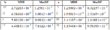
The biggest odds between two columns () and NDSolve are shown in Tab. 3. Therefore, we see that the biggest odds between two columns are very small.
u
n
x
i
Table 3. The biggest odds between two columns () and NDSolve of the MDE and the MmDE
u
n
x
i
4. Conclusions
4. Conclusions
The Mathieu’s equations were solved by the PSM. This method had accurately determined the numerical solutions for both cases a ⟶ 0 and large a. The accurate numerical computation is increasing if n is increasing. These numerical results proved that the PSM was good stable with respect to the large n.
Acknowledgments
Acknowledgments
The publication was prepared with the support of the “RUDN University Program 5-100”.
References
References
[1]. Gutierrez-Vega J. C., Rodriguez-Dagnino R. M., Mathieu functions, a visual approach, Am. J. Phys., 2003, 71(3), 233–242. doi: 10.1119/1.1522698.
[2]. Lawrence R., Applications of the Mathieu equation, Am. J. Phys., 1996, 64(1), 39–44. doi: 10.1119/1.18290.
[3]. Pomraning G. C., An Application of the Mathieu Equation to a Radiative Transfer Problem, SIAP, 1969, 17(6), 1065–1069, doi: 10.1137/0117096.
[4]. Kirkpatrick E. T., Tables of Values of the Modified Mathieu Functions, Mathematics of Computation, 1960, 14(70), 118–129, URL: https://www.jstor.org/stable/2003206.
[5]. Abramov A. A., Kurochkin S. V., Calculation of Solutions to the Mathieu Equation and of Related Quantities, Computational Mathematics and Mathematical Physics, 2007, 47(3), 397–406, doi: 10.1134/S0965542507030050.
[6]. Gadella M. H., Giacomini, L.P., Lara Periodic analytic approximate solutions for the Mathieu equation, Applied Mathematics and Computation, 2015, 271, 436–445, doi: 10.1016/j.amc.2015.09.018.
[7]. Hodge D. B., The calculation of the eigenvalues and eigenfunctions of Mathieu’s equation, NASA, 1972, ID: 19720007908, 15p, URL: https://ntrs.nasa.gov/search.jsp?R=19720007908.
[8]. Gheorghiu C. I., M. E. Hochstenbach, B. Plestenjak, J. Rommes, Spectral collocation solutions to multiparameter Mathieu’s system, Applied Mathematics and Computation, 2012, 218(24), 11990–12000, doi: 10.1016/j.amc.2012.05.068.
[9]. Samuel A. W., Nicolas V., Dmitry S. G., Jared H. C., Approximate solutions to Mathieu’s equation, Physica E: Low-dimensional Systems and Nanostructures, 2018, 100, 24–30, doi: 10.1016/j.physe.2018.02.019.
[10]. Mason J.C., Handscomb D.C., Chebyshev Polynomials, CRC Press LLC, 2003.
[11]. Trefethen Lloyd N., Spectral Methods in Matlab, SIAM, 2000.
[12]. Don W.S., Solomonoff A., Accuracy and speed in computing the Chebyshev collocation derivative, SISC, 1991, 16(6), 1253–1268.
[13]. Tinuade O., Abdolmajid M., Ousmane S., Application of the Chebyshev pseudospectral method to van der Waals fluids, Commun. Nonlinear Sci. Numer. Simulat., 2012, 17, 3499–3507, doi: 10.1016/j.cnsns.2011.12.025.
[14]. Arne Jensen, Lecture Notes on Spectra and Pseudospectra of Matrices and Operators, Aalborg University, 2009.
[15]. Martha L., Abell James P., Braselton Differential Equations with Mathematica, 3rd, Elsevier Inc, 2004.
Cite this as: Le Anh Nhat, "Pseudospectral Chebyshev method finds approximate solutions of the Mathieu’s equations" from the Notebook Archive (2019), https://notebookarchive.org/2019-11-2d1wasc
Download
