Educational Materials

Simplified Machine-Learning Workflow #1

Anton Antonov

Author

Anton Antonov

Title

Simplified Machine-Learning Workflow #1

Description

Quantile Regression (Part 1)

Quantile Regression monad examples

Live coding session aid

Anton Antonov
Accendo Data LLC

Wolfram Language live coding series
August 2019

In[]:=

Out[]=

Slide

Opening

The GitHub repository for this workshop

Mission statement.

The goals of this workshop are to introduce the theoretical background of Quantile Regression (QR), to demonstrate QR’s practical (and superior) abilities to deal with “real life” time series data, and to teach how to rapidly create QR workflows using Mathematica or R.

Slide

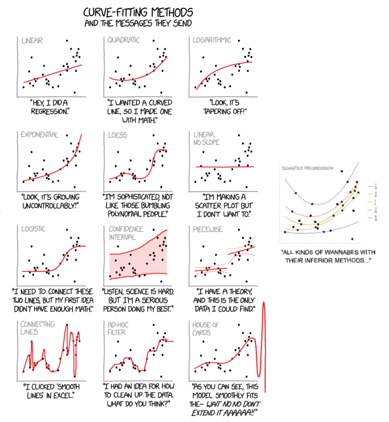
Quantile regression workflows

Out[]=

Slide

The software monad QRMon

When using a monad we lift certain data into the “monad space”, using monad’s operations we navigate computations in that space, and at some point we take results from it.

With the approach taken in this document the “lifting” into the QRMon monad is done with the function QRMonUnit. Results from the monad can be obtained with the functions QRMonTakeValue, QRMonContext, or with the other QRMon functions with the prefix “QRMonTake” (see below.)

Here is a corresponding diagram of a generic computation with the QRMon monad:

Out[]=

Remark: It is a good idea to compare the diagram with formulas (1) and (2).

Let us examine a concrete QRMon pipeline that corresponds to the diagram above. In the following table each pipeline operation is combined together with a short explanation and the context keys after its execution.

Out[]=

operation	explanation	context keys
QRMonUnit[tsData]⟹	lift data to the monad	{}
QRMonEchoDataSummary⟹	show the data summary	{}
QRMonQuantileRegression[12,{0.02`,0.98`}]⟹	do Quantile Regression with 12 knots	{data,regressionFunctions}
QRMonLeastSquaresFit[12]⟹	do Least Squares Fit with 12 polynomials	{data,regressionFunctions}
QRMonPlot⟹	plot data and regression functions	{data,regressionFunctions}
QRMonOutliers⟹	find outliers	{data,regressionFunctions,outliers,outlierRegressionFunctions}
QRMonOutliersPlot	plot data and outliers	{data,regressionFunctions,outliers,outlierRegressionFunctions}

Here is the output of the pipeline:

Data summary:

1 column 1

Min	3.62906× 9 10
1st Qu	3.65278× 9 10
Mean	3.67643× 9 10
Median	3.67645× 9 10
3rd Qu	3.70012× 9 10
Max	3.72375× 9 10

2 column 2

Min	5.89
1st Qu	19.695
Mean	22.2982
Median	23.33
3rd Qu	25.89
Max	31.17



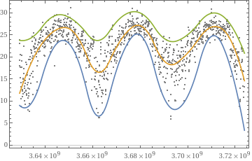
Plot:

	0.02
	0.98
	mean

Outliers plot:

The QRMon functions are separated into four groups:

◼

operations,

◼

setters and droppers,

◼

takers,

◼

State Monad generic functions.

An overview of the those functions is given in the tables in next two sub-sections. The next section, “Monad elements”, gives details and examples for the usage of the QRMon operations.

Monad functions interaction with the pipeline value and context


State monad functions


Slide

QRMon single line interpreter

Making a conversational agent for Quantile Regression workflows is my “end game.”

At this point I have programmed single line interpreters for variety of Machine Learning workflows.

One way to do it for Quantile Regression:

In[]:=

ToQRMonPipelineFunction["compute quantile regression using the quantiles 0.02, 0.98; show plot; display outliers plot"]

Out[]=

Function[{x,c},QRMonUnit[x,c]⟹QRMonQuantileRegression[6,{0.02,0.98},InterpolationOrder2]⟹QRMonPlot⟹QRMonOutliersPlot]

Another way to do it:

In[]:=

QRMonUnit[tsData]⟹ToQRMonPipelineFunction["show data summary"]⟹ToQRMonPipelineFunction["compute quantile regression with 10 knots and quantiles 0.02, 0.5 and 0.98"]⟹ToQRMonPipelineFunction["show plot"]⟹ToQRMonPipelineFunction["show outliers plot"];

Data summary:

1 column 1

Min	3.62906× 9 10
1st Qu	3.65278× 9 10
Mean	3.67643× 9 10
Median	3.67645× 9 10
3rd Qu	3.70012× 9 10
Max	3.72375× 9 10

2 column 2

Min	5.89
1st Qu	19.695
Mean	22.2982
Median	23.33
3rd Qu	25.89
Max	31.17



Plot:

	0.02
	0.5
	0.98

Outliers plot: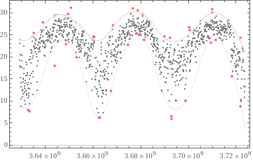

Random commands

In[]:=

ColumnForm@Union@GrammarRandomSentences[QRMonCommandsGrammar["Normalize"True],12]

Out[]=

calculate and display dataset outliers using from 390.775 to 390.775 using 390.775

calculate quantile regression

compute QuantileRegression

display dataset together with errors together with error , data , outlier , and dataset plot with date axis

do NetRegression using batch size 853.791 using batch size 853.791 over 853.791 hour using 853.791 rounds

find quantile regression over 224.278 together with 348.34 , and 348.34 , 348.34 , and 348.34 and 348.34 quantiles , and using the knots 102 , with from 471.06 to 873.585 by step 520.804 quantile

give plots with dates

make an standard workflow using EBNFNonTerminal[<classifier-algorithm>]

make a standard regression workflow

net regression

retrieve from context avmh25kl

use dataset that has id sdan

Slide

Simple pipelines

Using QR fit with the default B-splines basis.

In[]:=

QRMonUnit[distData]⟹QRMonQuantileRegression[12]⟹QRMonPlot;

Plot:

	0.25
	0.5
	0.75

In[]:=

QRMonUnit[tsData]⟹QRMonQuantileRegression[12,Range[0.1,0.9,0.2]]⟹QRMonDateListPlot[ImageSizeLarge];

Plot:

	0.1
	0.3
	0.5
	0.7
	0.9

Slide

Simple pipelines 2

We can make pipelines that compare QR fits with Linear Regression fits.

Here with QRMonFit we use the “default” Chebyshev polynomials basis.

In[]:=

QRMonUnit[distData]⟹QRMonQuantileRegression[12,0.5]⟹QRMonFit[5]⟹QRMonPlot[ImageSizeLarge];

Plot:

	0.5
	mean

Here we provide our own basis for QRMonFit.

In[]:=

QRMonUnit[distData]⟹QRMonQuantileRegression[12,0.5]⟹QRMonFit[Table[

,{i,0,7}]]⟹QRMonPlot[ImageSizeLarge];

Plot:

	0.5
	mean

Slide

Conditional CDF

One of the most powerful features of QR is the computation of conditional CDF’s (at specified regressor points.)

In[]:=

QRMonUnit[tsData]⟹QRMonQuantileRegression[12,Range[0.1,0.9,0.1]]⟹QRMonDateListPlot[ImageSizeLarge]⟹QRMonConditionalCDF[AbsoluteTime/@DateRange[{2016,1,1},{2017,1,1},Quantity[2,"Months"]]]⟹QRMonConditionalCDFPlot[PlotTheme"Detailed",ImageSizeMedium];

Plot:

	0.1
	0.2
	0.3
	0.4
	0.5
	0.6
	0.7
	0.8
	0.9

Conditional CDF's:3660595200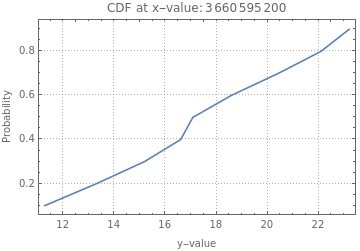

,3665779200

,3671049600

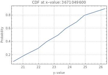,3676320000

,3681676800

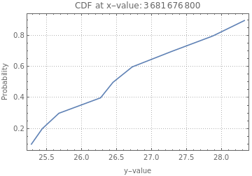,3686947200

,3692217600



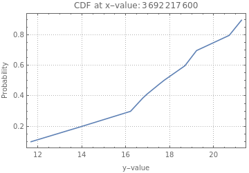
Slide

Outliers

Here we find contextual outliers.

In[]:=

QRMonUnit[tsData]⟹QRMonQuantileRegression[12,{0.02,0.98}]⟹QRMonOutliersPlot[ImageSizeLarge,"DateListPlot"True];

Outliers plot:

What we consider outlier can be manipulated by the smallest and larges regression quantiles.

In[]:=

QRMonUnit[tsData]⟹QRMonQuantileRegression[12,{0.3,0.95}]⟹QRMonOutliersPlot[ImageSizeLarge,"DateListPlot"True];

Outliers plot:

Slide

Errors

In[]:=

QRMonUnit[distData]⟹QRMonQuantileRegression[12]⟹QRMonPlot⟹QRMonErrorPlots⟹QRMonErrorPlots["RelativeErrors"False];

Plot:

	0.25
	0.5
	0.75

Relative error plots:0.25

,0.5

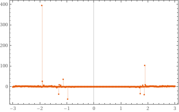,0.75



Error plots:0.25

,0.5

,0.75



Slide

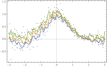
Over-training

Consider over-training your QR fits. That is similar to over-training Neural Networks.

In[]:=

QRMonUnit[distData]⟹QRMonQuantileRegression[50]⟹QRMonPlot;

Plot:

	0.25
	0.5
	0.75

In[]:=

QRMonUnit[distData]⟹QRMonQuantileRegression[100,0.5,InterpolationOrder1]⟹QRMonPlot;

Plot:

0.5

Slide

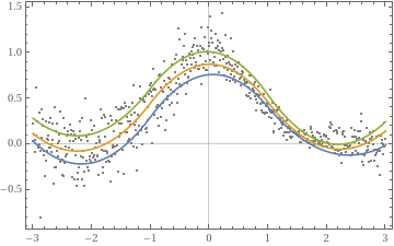
Getting out of the monad

Of course at some point we would want to get out of the monad and use the objects for further computations.

In[]:=

qFuncs=QRMonUnit[distData]⟹QRMonQuantileRegression[3,InterpolationOrder2]⟹QRMonPlot⟹QRMonTakeRegressionFunctions;

Plot:

	0.25
	0.5
	0.75

In[]:=

Simplify[#[x]]&/@qFuncs

Out[]=

0.25

-0.803994	x>3.\|\|x<-3.
1.44707-1.31693x+0.27687 2 x	1.≤x≤3.
0.761435+0.0543417x-0.408766 2 x	-1.≤x<1.
1.53996+1.61138x+0.369756 2 x	True

,0.5

-0.803994	x>3.\|\|x<-3.
1.63238-1.51119x+0.338479 2 x	1.≤x≤3.
0.874585+0.00440406x-0.419316 2 x	-1.≤x<1.
1.63195+1.51912x+0.338044 2 x	True

,0.75

-0.803994	x>3.\|\|x<-3.
1.82639-1.66699x+0.38013 2 x	1.≤x≤3.
1.01083-0.0358913x-0.435421 2 x	-1.≤x<1.
1.78165+1.50574x+0.335395 2 x	True



In[]:=

qrObj=QRMonUnit[distData]⟹QRMonQuantileRegression[12]⟹QRMonErrors;

In[]:=

Map[ListPlot,qrObj⟹QRMonTakeValue]

Out[]=

0.25

,0.5

,0.75



Slide

Quantile Regression vs shallow Neural Networks 1

Data

In[]:=

netDistData=Rule@@@RandomSample[distData,150];

In[]:=

plot=ListPlot[List@@@netDistData,PlotStyleRed]

Out[]=

Making the model net chain

In[]:=

NeuralNetworkGraph[<|"Input"3,"Hidden 1"8,"Hidden 2"8,"Output"1|>]

Out[]=

Input

Hidden 1

Hidden 2

Output

Create a multilayer perceptron with a large number of hidden units:

In[]:=

net=NetChain[{150,Tanh,150,Tanh,1}]

Out[]=

NetChain



uniniti

alized

Input port:	array
Output port:	vector (size: 1)
Number of layers:	5



Train the net for 10 seconds:

In[]:=

results1=NetTrain[net,netDistData,All,TimeGoal10]

Out[]=

NetTrain Results

summary

batches:14176,rounds:4726,time:10.0s,examples/s:90732

data

training examples:150,processed examples:907264,skipped examples:0

method

ADAMoptimizer,batch size64,CPU

round

loss:

2.69×

-2

	rounds
loss

Despite the noise in the data, the final loss is very low:

In[]:=

results1["FinalRoundLoss"]

Out[]=

Missing[KeyAbsent,FinalRoundLoss]

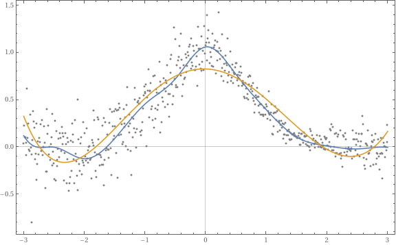
The resulting net overfits the data, learning the noise in addition to the underlying function. To see this, we plot the function learned by the net alongside the original data.

Obtain the net from the

NetTrainResultsObject

In[]:=

overfitNet=results1["TrainedNet"]

Out[]=

NetChain



Input port:	real
Output port:	scalar
Number of layers:	5



In[]:=

Show[Plot[overfitNet[x],{x,-3,3}],plot]

Out[]=

Slide

Quantile Regression vs shallow Neural Networks 2

Quantile regression computation

Similarities:

◼

Hidden layer nodes ↔ Knots

◼

Tanh, ReLU ↔ B-Spline, interpolation order

Slide

Quantile Regression vs shallow Neural Networks 3

Interactive over-fitting

In[]:=

DynamicModule[{qs,qFuncs,knots,data=netDistData},Manipulate[qs={0.25,0.5,0.75};(*qFuncs=QRMonUnit[List@@@data]⟹QRMonQuantileRegression[nKnots,qs,InterpolationOrderintOrder]⟹QRMonTakeRegressionFunctions;*)qFuncs=QuantileRegression[List@@@data,nKnots,qs,InterpolationOrderintOrder];knots=Rescale[Range[0,1,1/nKnots],{0,1},{Min[data[[All,1]]],Max[data[[All,1]]]}];Show[{ListPlot[List@@@data,PlotStyleRed,GridLines{If[showKnotsQ,knots,None],None},GridLinesStyleDirective[GrayLevel[0.8],Dashed]],Plot[Through[qFuncs[x]],{x,Min[data〚All,1〛],Max[data〚All,1〛]},PerformanceGoal"Speed"]}],{{nKnots,12,"number of knots:"},0,100,1},{{intOrder,2,"interpolation order:"},1,12,1},{{showKnotsQ,False,"show knots:"},{False,True},ControlTypeCheckbox}]]

Out[]=

number of knots:

interpolation order:

show knots:

Slide

Anticipated questions at this point

How the computations are done?

Why use monadic programming / pipelining?

How to choose the right basis functions?

What if I want to basis functions other than B-Splines?

Slide

Using monads for conversational agents

The use of monadic DSL’s big picture.

In[]:=

Slide

Initialization code

Load main packages

In[]:=

Import["https://raw.githubusercontent.com/antononcube/MathematicaForPrediction/master/MonadicProgramming/MonadicContextualClassification.m"];Import["https://raw.githubusercontent.com/antononcube/MathematicaForPrediction/master/MonadicProgramming/MonadicQuantileRegression.m"];Import["https://raw.githubusercontent.com/antononcube/MathematicaForPrediction/master/MonadicProgramming/MonadicNeuralNetworks.m"];Import["https://raw.githubusercontent.com/antononcube/MathematicaForPrediction/master/MonadicProgramming/MonadicTracing.m"]

Importing from GitHub:MathematicaForPredictionUtilities.m

Importing from GitHub:MosaicPlot.m

Importing from GitHub:CrossTabulate.m

Importing from GitHub:ParetoPrincipleAdherence.m

Importing from GitHub:StateMonadCodeGenerator.m

Importing from GitHub:ClassifierEnsembles.m

Importing from GitHub:ROCFunctions.m

Importing from GitHub:VariableImportanceByClassifiers.m

Importing from GitHub:SSparseMatrix.m

Importing from GitHub:OutlierIdentifiers.m

Importing from GitHub:QuantileRegression.m

Load data

In[]:=

Import["https://raw.githubusercontent.com/antononcube/MathematicaVsR/master/Projects/ProgressiveMachineLearning/Mathematica/GetMachineLearningDataset.m"]

In[]:=

Needs["GetMachineLearningDataset`"];dsTitanic=GetMachineLearningDataset["Titanic"];dsMushroom=GetMachineLearningDataset["Mushroom"];dsWineQuality=GetMachineLearningDataset["WineQuality"];

Distribution data

The following data is generated to have heteroscedasticity.

In[]:=

distData=Tablex,Exp[-x^2]+RandomVariateNormalDistribution0,.15

Abs[1.5-x]/1.5

,{x,-3,3,.01};QRMonUnit[distData]⟹QRMonEchoDataSummary⟹QRMonPlot;

Data summary:

1 Regressor

Min	-3.
1st Qu	-1.5025
Median	0.
Mean	7.98031× -17 10
3rd Qu	1.5025
Max	3.

2 Value

Min	-0.495278
1st Qu	0.0220022
Median	0.184354
Mean	0.294181
3rd Qu	0.560785
Max	1.28074



Plot:

Temperature data

In[]:=

tsData=WeatherData[{"Orlando","USA"},"Temperature",{{2015,1,1},{2018,1,1},"Day"}]QRMonUnit[tsData]⟹QRMonEchoDataSummary⟹QRMonDateListPlot;

Out[]=

$Aborted

GetData:Cannot find data.

QRMonBind:Failure when applying: QRMonGetData

QRMonBind:Failure when applying: QRMonEchoDataSummary

Financial data

In[]:=

finData=TimeSeries[FinancialData["NYSE:GE",{{2014,1,1},{2018,1,1},"Day"}]];QRMonUnit[finData]⟹QRMonEchoDataSummary⟹QRMonDateListPlot;

RecordsSummary

::arrdepth

:The first argument is expected to be a full array of depth 1 or 2.

Data summary:$Failed

GetData:Cannot find data.

QRMonBind:Failure when applying: QRMonDateListPlot

Neural network construction

In[]:=

ClearAll[NeuralNetworkGraph]NeuralNetworkGraph[layerCounts:{_Integer..}]:=NeuralNetworkGraph[AssociationThread[Row[{"layer ",#}]&/@Range@Length[layerCounts],layerCounts]];NeuralNetworkGraph[namedLayerCounts_Association]:=Block[{graphUnion,graph,vstyle,layerCounts=Values[namedLayerCounts],layerCountsNames=Keys[namedLayerCounts]},graphUnion[g_?GraphQ]:=g;graphUnion[g__?GraphQ]:=GraphUnion[g];graph=graphUnion@@MapThread[IndexGraph,{CompleteGraph/@Partition[layerCounts,2,1],FoldList[Plus,0,layerCounts[[;;-3]]]}];vstyle=Catenate[Thread/@Thread[TakeList[VertexList[graph],layerCounts]ColorData[97]/@Range@Length[layerCounts]]];graph=Graph[graph,GraphLayout{"MultipartiteEmbedding","VertexPartition"layerCounts},GraphStyle"BasicBlack",VertexSize0.5,VertexStylevstyle];Legended[graph,Placed[PointLegend[ColorData[97]/@Range@Length[layerCounts],layerCountsNames,LegendMarkerSize30,LegendLayout"Row"],Below]]];

Cite this as: Anton Antonov, "Simplified Machine-Learning Workflow #1" from the Notebook Archive (2020), https://notebookarchive.org/2020-09-55roh1k

Quantile Regression monad examples

Live coding session aid

Opening

Mission statement.

Quantile regression workflows

The software monad QRMon

Monad functions interaction with the pipeline value and context

State monad functions

QRMon single line interpreter

Random commands

Simple pipelines

Simple pipelines 2

Conditional CDF

Outliers

Errors

Over-training

Getting out of the monad

Quantile Regression vs shallow Neural Networks 1

Data

Making the model net chain

Quantile Regression vs shallow Neural Networks 2

Quantile regression computation

Quantile Regression vs shallow Neural Networks 3

Interactive over-fitting

Anticipated questions at this point

Using monads for conversational agents

Initialization code

Load main packages

Load data

Distribution data

Temperature data

Financial data

Neural network construction

Monad functions interaction with the pipeline value and context


State monad functions
