The Quantum Harmonic Oscillator in the Wolfram Physics Model
Author
Patrick Geraghty
Title
The Quantum Harmonic Oscillator in the Wolfram Physics Model
Description
A description of how the Quantum Harmonic Oscillator can be represented by periodic multiway systems in the Wolfram Physics Model.
Category
Essays, Posts & Presentations
Keywords
URL
http://www.notebookarchive.org/2020-07-6hj3mxm/
DOI
https://notebookarchive.org/2020-07-6hj3mxm
Date Added
2020-07-14
Date Last Modified
2020-07-14
File Size
0.51 megabytes
Supplements
Rights
Redistribution rights reserved

WOLFRAM SUMMER SCHOOL 2020
The Quantum Harmonic Oscillator in the Wolfram Fundamental Physics Model
The Quantum Harmonic Oscillator in the Wolfram Fundamental Physics Model
Patrick Geraghty
Utrecht University
One of the most fundamental systems in quantum mechanics is the quantum harmonic oscillator. The key attribute of the quantum harmonic oscillator is the quantization of the energy levels within the oscillator and their relation to the frequency of the energy level. In order to find the QHO in the Wolfram Fundamental Physics Model, these same principal attributes must be found. In this project, string substitution multiway systems that are periodic in time are used. The ladder operators, position operator, energy eigenstates, and a potential route for complex phases are found along with other key elements of the quantum harmonic oscillator.
Wolfram Community Post
Wolfram Community Post
What is Periodicity in a Multiway System?
What is Periodicity in a Multiway System?
The key attribute of the harmonic oscillator is periodicity; before even taking into account the quantum nature of the system examined here, first, periodicity is needed. This is defined as a system that starts in a beginning state, S, and then evolves in time, returning to the initial state S, and repeating the cycle again. In the Wolfram Physics Model, this can be represented with a string substitution method of forming multiway graphs where the systems have a cyclical pattern.
In[]:=
{LayeredGraphPlot[ResourceFunction["MultiwaySystem"][{"S""A","A""S"},{"S"},2,"EvolutionGraph"],Left],LayeredGraphPlot[ResourceFunction["MultiwaySystem"][{"S""A","A""B","B""S"},"S",3,"EvolutionGraph"],Left]}
Out[]=
{ ,
, }
}
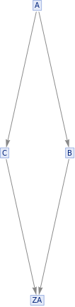
The two multiway systems shown above are both periodic in time because they continually return to the initial state S, however, they both have different periods. The energy of a multiway system is hypothesized to be proportional to the flux of causal lines through timelike hypersurfaces. The second system above has a longer period and a longer period means that there is a greater flux of causal lines and thus more energy in the system. From here, our hypothesis is that the period of a multiway system is proportional to the energy and thus frequency of the quantum harmonic oscillator.
Results
Results
In[]:=
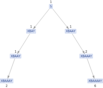
ResourceFunction["MultiwaySystem"][{"BA""AB","BY""CY","AC""CA","XC""XB"},{"XBAAAY"},10,"StatesGraph"]
Out[]=

The multiway graph shown above uses X and Y as boundaries and A as a placeholder related to the period. The system begins with XBAAAY and the time evolution moves the B from the left-hand side to the right-hand side. When the B reaches the Y side it turns into a C and returns the other direction. The time evolution as the B/C move across the string and back is the period of the cycle. Naturally as the number of A’s increases, the period increases by an additive factor of 2:
In[]:=
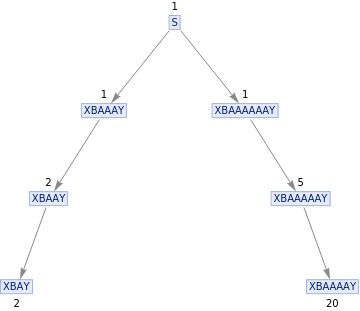
ResourceFunction["MultiwaySystem"][{"BA""AB","BY""CY","AC""CA","XC""XB"},{"XBAY"},5,"StatesGraph"]
Out[]=

The starting state given above, XBAY, is taken to be the ground state of the quantum harmonic oscillator with n=0. The convenient part of this particular system is that the same rules can be used for any period or number of A’s in place.
Energy
Energy
In the standard quantum harmonic oscillator, the energy spectrum should follow the relation: In this standard format, the difference in energy between each successive level is two times the zero point energy. The difference in period between successive multiway systems is half the period of the ground state. Given the ansatz that energy is proportional to the period of a multiway system, there is a discrepancy in the role of the ground state that needs to be addressed in future workIt is believed that this represents the quantum harmonic oscillator because it matches the key attributes that are known about the QHO; a discrete energy spectrum with values linearly proportional to the energy of each level. However, the period of the multiway system is not necessarily directly the same as the period of a physical system, it is a model that yields similar characteristics.
Ladder Operators
Ladder Operators
The ladder operators, or the creation and annihilation operators, are very important in the quantum harmonic oscillator because they are the operators that send one energy eigenstate to either the next up or next below energy eigenstate. Using the same definition of the states with the bouncing letters from above, these ladder operators can be seen as a string substitution rule. The creation operator is the rule “A” -> ”AA”, and the annihilation operator rule is “AA” -> “A”.
In[]:=
{ResourceFunction["MultiwaySystem"][{"A""AA","S""XBAY","S""XBAAY"},{"S"},3,"EvolutionGraph","IncludeStatePathWeights"True,VertexLabels"VertexWeight"],ResourceFunction["MultiwaySystem"][{"AA""A","S""XBAAAY","S""XBAAAAAAY"},{"S"},3,"EvolutionGraph","IncludeStatePathWeights"True,VertexLabels"VertexWeight"]}
Out[]=
 ,
,
In the standard formulation of quantum mechanics, the ladder operators act on an energy eigenstate with the relations below are the result. The vertex weights shown at each label are follow rules shown below:
 The discrepancy between these two relations is unclear, however given that the vertex weights are almost nearly the same values as those from the energy eigenstate relations, it is unlikely to be coincidence. The extra square root value comes from the definition of the number operator where N |n > = n |n >, and N can be written as the product of the creation and annihilation operators. It is possible that the square root may need to be inserted for consistence.Another attribute of the ladder operators that can be nearly replicated is the commutation relation between the creation and annihilation operators. When the commutator is equal to zero, this means that the resulting state is independent of the order in which the operators are applied. In the case of the standard ladder operators the difference should just be a factor of 1.
In[]:=
ResourceFunction["MultiwaySystem"][{"A""AA","AA""A","S""XBAAAY"},{"S"},3,"EvolutionGraph","IncludeStatePathWeights"True,VertexLabels"VertexWeight","IncludeStateID"True]
Out[]=

The commutator between the creation and annihilation operators is shown in the strong diamond convergence shown above. The left side of the diamond first operates creation to send XBAAAY to XBAAAAY, with a vertex weight of 3, and then the annihilation operator to send XBAAAAY back to XBAAAY. The right side of the diamond acts annihilation first, a vertex weight of 2, and then creation to bring the system back to the original XBAAAY. The vertex weight in the resulting XBAAAY is 13 because the vertex weights of the resulting XBAAAY from each side are added together; the left weight is 9 and the right weight is 4. However, the commutator subtracts the two operations which results in a weight of 5. This value matches the ladder operator relations for a multiway system as shown above because the multiway system has the commutator shown below. where n is directly related to the period of the beginning state, in this case XBAAAY which has n = 2.
Conclusion and Phase
Conclusion and Phase
With the periodic structure and the ladder operators defined, the multiway system below shows the operations of both time evolution and the ladder operators. Each cyclic petal from the center has a different period and thus a different energy associated with it, where the shortest period shown represents the ground state energy of the quantum harmonic oscillator. The arrows around the center show all of the allowed transitions between energy levels for each of the beginning states. Note that there are no arrows between XBAY an XBAAAY because only a jump of +/- 1 is allowed.
In[]:=
ResourceFunction["MultiwaySystem"][{"BA""AB","BY""CY","AC""CA","XC""XB","S""XBAY","S""XBAAY","S""XBAAAY","XBAY""XBAAY","XBAAY""XBAY","XBAAAY""XBAAY","XBAAY""XBAAAY"},{"S"},9,"StatesGraph"]
Out[]=

In terms of next steps, a potential method for defining the phase difference between given energy eigenstates has been partially developed but not completed. The phase difference is defined qualitatively as the ratio of the branchlike to spacelike separated events. In the case above, each of the states within a cycle are spacelike separated which contributes a phase factor of 0. Each petal, however, is branchlike separated and this yields a non-zero phase factor.
The non-zero phase factor picked up by branchlike separated events is theorised to be proportional to the difference in the path length of the cycle. This would yield a statement such as Δθ = c Δl, where c is some constant that describes the relationship between phase difference and path length difference. The phase would then be written as exp[i π Δθ] = exp[i π cΔl]. This structure of the phase difference is a potential method but requires more study to truly be consistent with the system.
The non-zero phase factor picked up by branchlike separated events is theorised to be proportional to the difference in the path length of the cycle. This would yield a statement such as Δθ = c Δl, where c is some constant that describes the relationship between phase difference and path length difference. The phase would then be written as exp[i π Δθ] = exp[i π cΔl]. This structure of the phase difference is a potential method but requires more study to truly be consistent with the system.
Next Steps
Next Steps
The next steps include diving deeper into developing a more concrete way of evaluating the path integral in a periodic multiway system. The path integral is defined as the sum over all paths and the bifurcations shown through a period can be seen as different paths that would be summed over; each path through the system is a geodesic.
One of the most important next steps is to get a more concrete, calculatable definition of the energy in the system. The energy is define as the flux of edges in a multiway causal graph through timelike hypersurfaces. When looking at periodicity in space, instead of the timelike periodicity discussed here, the energy differences are made more obvious.
One of the most important next steps is to get a more concrete, calculatable definition of the energy in the system. The energy is define as the flux of edges in a multiway causal graph through timelike hypersurfaces. When looking at periodicity in space, instead of the timelike periodicity discussed here, the energy differences are made more obvious.
In[]:=
ResourceFunction["MultiwaySystem"][{"A""A","B""B","C""C","D""D","E""E","F""F","G""G","H""H","I""I","S""ABC","S""DE","S"->"FHGI"},"S",3,"EvolutionCausalGraph","IncludeStepNumber"True]
Out[]=

Here the flux of the orange causal edges increases linearly by a factor of two for each extra spacelike branch. Examining these spacelike periodic systems certainly appears worth the work in the future.
Complete project work
Complete project work
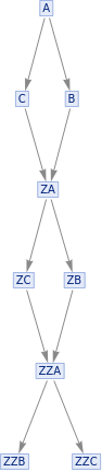
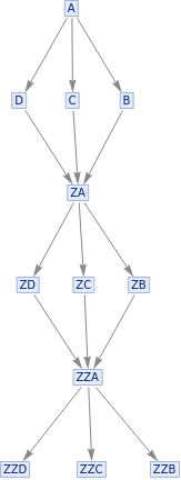
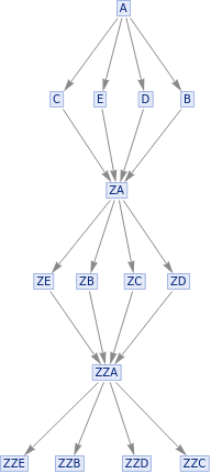
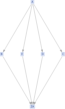
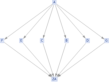
This is a series of period 2 systems with different widths. Energy is define as flux of causal lines through timelike hypersurfaces; here the energy alternates from step to step and increases with width. Following the ansatz that period is proportional to energy it is odd not only that the energy is not constant but also that for the same period different energies can be seen.
In[]:=
{ResourceFunction["MultiwaySystem"][{"A""B","A""C","B""ZA","C""ZA"},{"A"},5,"CausalGraph"],ResourceFunction["MultiwaySystem"][{"A""B","A""C","B""ZA","C""ZA"},{"A"},5,"EvolutionGraph"]}{ResourceFunction["MultiwaySystem"][{"A""B","A""C","A""D","B""ZA","C""ZA","D""ZA"},"A",5,"CausalGraph"],ResourceFunction["MultiwaySystem"][{"A""B","A""C","A""D","B""ZA","C""ZA","D""ZA"},"A",5,"EvolutionGraph"]}{ResourceFunction["MultiwaySystem"][{"A""B","A""C","A""D","A""E","B""ZA","C""ZA","D""ZA","E""ZA"},"A",5,"CausalGraph"],ResourceFunction["MultiwaySystem"][{"A""B","A""C","A""D","A""E","B""ZA","C""ZA","D""ZA","E""ZA"},"A",5,"EvolutionGraph"]}
Out[]=
 ,
,
Out[]=
 ,
,
Out[]=
 ,
,
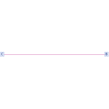
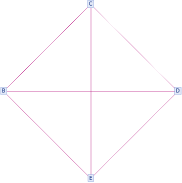
There is an interesting pattern in branchial space where the the width of the graph will show different complete graphs for different widths. It makes sense given that a complete graph is defined as a graph where all vertices are connected to all other vertices.
In[]:=
{ResourceFunction["MultiwaySystem"][{"A""B","A""C","B""ZA","C""ZA"},{"A"},1,"BranchialGraph"],ResourceFunction["MultiwaySystem"][{"A""B","A""C","B""ZA","C""ZA"},{"A"},2,"EvolutionGraph"]}{ResourceFunction["MultiwaySystem"][{"A""B","A""C","A""D","B""ZA","C""ZA","D""ZA"},"A",1,"BranchialGraph"],ResourceFunction["MultiwaySystem"][{"A""B","A""C","A""D","B""ZA","C""ZA","D""ZA"},"A",2,"EvolutionGraph"]}{ResourceFunction["MultiwaySystem"][{"A""B","A""C","A""D","A""E","B""ZA","C""ZA","D""ZA","E""ZA"},{"A"},1,"BranchialGraph"],ResourceFunction["MultiwaySystem"][{"A""B","A""C","A""D","A""E","B""ZA","C""ZA","D""ZA","E""ZA"},{"A"},2,"EvolutionGraph"]}{ResourceFunction["MultiwaySystem"][{"A""B","A""C","A""D","A""E","A""F","B""ZA","C""ZA","D""ZA","E""ZA","F""ZA"},{"A"},1,"BranchialGraph"],ResourceFunction["MultiwaySystem"][{"A""B","A""C","A""D","A""E","A""F","B""ZA","C""ZA","D""ZA","E""ZA","F""ZA"},{"A"},2,"EvolutionGraph"]}{ResourceFunction["MultiwaySystem"][{"A""B","A""C","A""D","A""E","A""F","A""G","B""ZA","C""ZA","D""ZA","E""ZA","F""ZA","G""ZA"},{"A"},1,"BranchialGraph"],ResourceFunction["MultiwaySystem"][{"A""B","A""C","A""D","A""E","A""F","A""G","B""ZA","C""ZA","D""ZA","E""ZA","F""ZA","G""ZA"},{"A"},2,"EvolutionGraph"]}
Out[]=
 ,
,
Out[]=
 ,
,
Out[]=
 ,
,
Out[]=
 ,
,
Out[]=
 ,
,
The systems described in the main body of work are all of width 1. The figures above both show that there are some interesting dynamics created with other widths of divergence that needs more examination.
Keywords
Keywords
◼
Harmonic Oscillator
◼
Quantum
◼
Multiway System
◼
Operators
Acknowledgment
Acknowledgment
Mentor: Kiel Howe
I would like to acknowledge my Kiel Howe for all of his help and ideas throughout this project. I would like to acknowledge Jonathan Gorard for his advice on the new directions within the project and his patience. I would like to thank Stephen Wolfram for making this project possible. Lastly, I would like to thank the entire Wolfram Summer School students and staff for making this virtual system work so well and for making this new era of collaboration a real success.
References
References
◼
Bohm, David. Quantum Theory. New York, Prentice Hall, 1951.
◼
Andrew Dotson. “Deriving the Feynman Path Integral Parts 1 and 2.” Youtube.com, June 2019, August 2019. https://www.youtube.com/watch?v=XCsIfkFd1aE. July 10th, 2020.
Cite this as: Patrick Geraghty, "The Quantum Harmonic Oscillator in the Wolfram Physics Model" from the Notebook Archive (2020), https://notebookarchive.org/2020-07-6hj3mxm
Download
