Weyl’s Law And The Wolfram Model Of Physics

Jon Lederman

Spinor

The goal of this work is explore Weyl’s Law as it may relate to the graphs underlying the Wolfram Model of Physics. Weyl’s law describes the nature of the asymptotic growth of the eigenvalues of the Laplacian operator on bounded domains having Dirichlet and Neumann boundary conditions. The Laplace-Beltrami operator is a generalization of the Laplacian for operating on Riemannian manifolds. In the context of the Wolfram Model of physics, an ongoing area of investigation is whether the principles of Einstein’s theory of General Relativity thereby arise as emergent phenomena. As General Relativity is described in the language of Riemannian Geometry, the question of whether properties of Riemannian manifolds also hold on these graphs. Weyl’s law is a statement regarding the asymptotic growth of the eigenvalues of the Laplacian on bounded domains with DIrichlet or Neumann boundary conditions. The law has been extended to non-Euclidean space through a generalization of the Laplace operator called the Laplace-Beltrami operator. This investigation of Weyl’s law in the context of the Wolfram Model posits a number of fundamental questions at the intersection of Riemannian geometry and graph theory, among which a principal question is what the appropriate analogue for the Laplace-Beltrami operator is for digraphs. In particular, does there exist a generalization of the graph Laplacian that encodes geometric information in the Wolfram model graphs analogous to Laplace-Beltrami operator on Riemannian manifolds?

Wolfram Community Post

Introduction

The rest of this work will be arranged as follows: 1. Heat Kernel on Graphs Part 1 will develop the theory and associated code in Mathematica for implementing the partial differential equation describing heat diffusion (i.e., the heat equation) on graphs. The motivation for this focus is to (a) explore issues relating to the mapping of continuous PDEs to discrete graph structures with respect to preserving the underlying physics; (b) explore how the representation of PDEs on graphs and spectral graph theory may illuminate various geometric attributes of these discrete structures including dimension and curvature. The computational aspects of this work will include development of code for performing temporal evolution of the heat equation from some initial conditions as well as visualization tools for studying the behavior of heat diffusion on graphs. 2. Weyl’s Law on Graphs Part 2 will introduce Weyl’s law and its interpretation as well as its application to a number of branches of physics, acoustics and of course Riemannian manifolds. The computational work in this section will examine whether any correspondence can be ascertained between the spectrum of the graph Laplacian and of the effective definition of dimension of a graph as defined in the Wolfram Physics Model. 3. The Laplace-Beltrami Operator Part 3 will examine approaches for developing and analog of the Laplace-Beltrami operator for graphs. First, we will provide a derivation of the functional form of the operator for continuous manifolds. Next, we will provide some analysis and thoughts regarding approaches for generalizing the Laplace-Beltrami operator on graphs. 4. Spectral Graph Theory and Future Work Part 4 will discuss some ideas in spectral graph theory and miscellaneous ideas for future work in further analyzing this problem.

1. The Heat Equation

The Heat Equation PDE

The heat equation

is a partial differential equation describing the time evolution of the diffusion in space of a physical quantity such as heat. α is a constant referred to as the thermal diffusivity. Interestingly, the Schrodinger equation bears some relationship to the heat equation in that it is 2nd order in space and first order in time although it introduces an imaginary coefficient in the time dependence. Linear operator equations such as the heat equation may be solved by several different methods. One method involves finding the Green’s function for the heat equation (the heat kernel). A Green’s function effectively describes the response function to a point source in time, space or both. The total response may then be determined by calculating the linear superposition of responses for an initial condition. Alternatively, the solution to the heat equation for some initial conditions may be determined by the following method: 1) Calculate the eigenvalues and eigenfunctions of the Laplacian operator; 2) Project the initial conditions onto the eigenspace using the determined eigenvectors to generate a set of eigenspace coordinates; 3) Perform the temporal evolution in the eigenspace for each eigenvector using the associated eigenvalue and projection coordinates. Because by definition, the operator is diagonal in the eigenspace coordinates, carrying out the time evolution will be a decoupled trivial exponential; 4) Upon evolving each eigen - component in the eigenspace, project back to the temperature space.We choose the latter approach. In particular, as we seek to encode the heat equation to a graph, we will derive the analogous discrete operator on a graph, the Laplacian matrix, which we turn to next.

Discretizing the Heat Equation

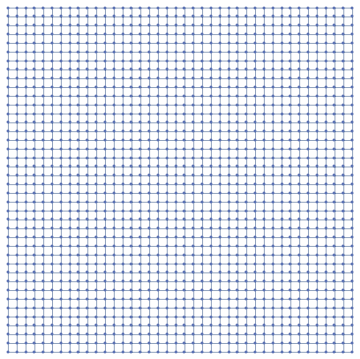
How can we map the heat equation to a graph? Formally, a graph comprises a set of vertices connected via a series of edges. Our end goal is to study the behavior of the Laplacian and it’s generalization to non-Euclidean spaces, the Laplace-Beltrami operator with respect to graphs generated via the evolutionary application of rules as defined in the Wolfram Model. For now, however, Imagine a simple planar graph such as the following :

In[]:=

simpleGridGraph=GridGraph[{16,16},VertexSizeLarge]

Out[]=

Each vertex may associated with a temperature, such that the composite set of temperatures defines a heat distribution on the graph. We can define a temperature or heat distribution function ϕ(v) that maps a temperature to each vertex. For visualization purposes, we can indicate the temperature on a graph using color. To do so, let’s define some functions to color our graph based upon the temperature at each vertex. As our immediate goal is to model the temporal evolution of heat flow based upon the heat equation, We will use these coloring functions later visualizing the heat flow on more complex graphs such as those arising in the Wolfram Model.

In[]:=

(*TakesagraphandtemperaturesandsetsthetemperaturesonthegraphastheVertextWeight*)Attributes[SetTemperatures]={HoldFirst};SetTemperatures[g_,temperatures_]:=AnnotationValue[g,VertexWeight]=temperatures;(*TakesagraphandtemperaturesandsetsthetemperaturesonthegraphastheVertextWeightreturninganewgraph*)SetTemperaturesNG[g_,tmps_]:=Module[{ng=g},AnnotationValue[{ng},VertexWeight]=tmps;ng];(*Returnsthetemperaturesonagraph*)GetTemperatures[g_]:=AnnotationValue[g,VertexWeight];(*Createsarandomtemperaturedistributiononagraph*)ColorByRandomTemperature[g_]:=ColorByTemperature[g,Table[RandomReal[],VertexCount[g]]];(*Colorsagraphusingatemperaturelist*)ColorByTemperature[g_,temperatures_]:=HighlightGraph[g,MapThread[Style,{VertexList[g],Map[ColorData["Rainbow"],temperatures]}]];(*Colorsagraphbyitsinternaltemperatures(fromalreadyassignedVertexWeights)*)ColorByInternalTemperature[g_]:=ColorByTemperature[g,GetTemperatures[g]];

Let' s apply a random temperature distribution to our simple grid graph for illustrative purposes :

In[]:=

ColorByRandomTemperature[simpleGridGraph]

Out[]=

We are using the Rainbow color scheme as defined in Mathematica, but are free to choose other schemes. The Rainbow scheme maps purple to the coldest temperature and red to the hottest :

In[]:=

ColorData["Rainbow"]

Out[]=

ColorDataFunction

Name: Rainbow

Gradient:



We can further imagine that a vertex coupling two vertices allows heat to flow directly between the two vertices. On the other hand, if two vertices are not directly connected no heat can directly flow, but instead may flow through some other path if the vertices are connected through some other set of vertices. Since we are seeking to model the temporal evolution of heat diffusion, we will necessarily define some initial conditions on our graph. Although the random distribution looks pretty, it' s not particularly realistic for what we might expect of our initial conditions. Instead, we seek something like a delta function wherein our heat distribution is characterized by a concentrated heat source. In order to do that, we will define some functionality to generate a a rough delta or point source distribution on our graph. While we’re at it, let’s also define some functionality to normalize temperatures between 0-1 so that we can conviently apply a color map.

In[]:=

(*Setsadeltafunctiononagraphatvertexofsizedistance*)SetDeltaFunction[g_,vertex_,distance_]:=Module[{ng=g},(AnnotationValue[{ng,#},VertexWeight]=ConstantArray[1,Length[#]])&@VertexList[NeighborhoodGraph[g,vertex,distance]];ng];(*Normalizestemperaturesonagraphbetween0and1*)Attributes[NormalizeTemperatures]={HoldFirst};NormalizeTemperatures[g_]:=SetTemperatures[g,N[#/Max[#]]]&@GetTemperatures[g];(*Normalizesavectorofinitialconditions*)NormalizeConditions[ic_]:=N[ic/Max[ic]];(*Zerosoutthetemperaturedistribution*)MakeUniformlyCold[g_]:=SetTemperatures[g,ConstantArray[0,VertexCount[g]]];

Let' s now clear our temperature distribution on simpleGridGraph and instead impose a delta function like initial condition:

In[]:=

SetTemperatures[simpleGridGraph,ConstantArray[0,256]];ColorByInternalTemperature[simpleGridGraph];deltaGridGraph=SetDeltaFunction[simpleGridGraph,135,3];ColorByInternalTemperature[deltaGridGraph]

Out[]=

Now we are set up to represent temperatures on our graph and define delta - like initial conditions. But, we are yet to attack the most important question of how to perform temporal evolution of the heat equation on the graph. In short, we will discretize over space but leave the time dependence as a continuous variable. In order to do that, we need to define the adjacency matrix A for our graph. If we define a matrix in which each row index corresponds to a vertex in the graph and similarly, each column, we define the entry for each row as 0 if an edge exists between the respective vertices indexed by the row and column. Thus, if we have N vertices in the graph, the adjacency matrix is an N*N matrix of 1’s and 0’s indicating whether particular vertices are connected to one another.

The final step in encoding the heat equation PDE to a graph is to figure out how to model the Laplacian operator itself. A simple approach is to recognize physically that the rate of heat diffusion at a given vertex with respect an adjacent vertex by Newton’s law of cooling is proportional to the difference in temperature between the adjacent vertices assuming the temperature differential is small. Alternatively, we could have evaluated the discrete difference approximation to the second derivative using a numerical approximation scheme. This approach would yield a central difference approximation with a dependence upon the inverse square of the discrete distance between adjacent nodes. In our scheme, adjacent vertices are assumed to have a unit distance. However, because of complications involving applying the central difference approximation to graphs, we choose the former approach.

We are now ready to write down our discretized heat equation on a graph. In words, the time derivative of the temperature of each vertex equals the linear superposition of temperature differences between ALL adjacent nodes.

For purposes of this discussion, we will normalize α to 1. We can now manipulate this equation as follows. The operator ' deg' shown below calculates the number of outgoing or equivalently incoming vertices to a given vertex. In the end we arrive with a discrete operator equation for a new operator L, which represents the discrete Laplacian operator for our graph. After some derivation as follows, the Laplacian matrix emerges as the appropriate operator for the heat equation on a graph:

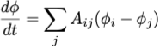
Here D is a diagonal matrix wherein each entry on the diagonal counts the number of outgoing (or equivalently incoming) edges for a vertex. In essence, we are left with a simple one-dimensional homogeneous ordinary differential equation in time.

It is understood here that ϕ is a vector of temperature coefficients defining the heat distribution on the graph. In our case, we seek to solve the this equation in which we define some initial conditions specifying the temperature distribution at time 0. As noted previously, this equation can be solved by standard techniques for ODEs by projecting the initial conditions onto the eigenspace, performing the temporal evolution there and projecting back again to temperature space. And indeed that is what we shall do as codified in the following Wolfram Language code. First, let’s calculate the graph associated matrices such as the adjacency matrix and the Laplacian matrix:

In[]:=

(*ThefollowingcodecalculatesthegraphLaplaciananditsspectrum.UnnormalizedLaplacianreturnstheunnormalizedLaplacianoftheassociatedundirectedgraph.AdjMatrixconvertsadirectedgraphtoanundirectedgraphandcalculatestheadjacencymatrix.GraphSpectrumreturnstheeigenvaluesandeigenfunctionsofthegraphinputobjectasanassociativearray.*)UnnormalizedLaplacian[g_]:=N@(DiagonalMatrix[VertexOutDegree[#]]-AdjacencyMatrix[#])&@UndirectedGraph[g];AdjMatrix[g_]:=N@AdjacencyMatrix[#]&@UndirectedGraph[g];GraphSpectrum[g_]:=<|"eigenvalues"->Eigenvalues[#],"eigenvectors"->Eigenvectors[#]|>&@UnnormalizedLaplacian[g];

The next set of code performs the heat kernel dynamics using the above described approach of eigenvector decomposition.

In[]:=

(*Thefollowingcodeimplementstheheatkerneldynamics.*)(*Projectinitialconditionsontoeigenspace*)EigenSpaceProject[ic_,eigenvectors_]:=eigenvectors.ic;(*Projectvector,whichmaybeatimeevolvedvectorineigenspaceontovertexspace(temperaturespace)*)VertexSpaceProject[vector_,eigenvectors_]:=Transpose[eigenvectors].vector;(*Performtemporalevolutionineigenspace*)EigenSpaceAdvance[spectrum_,coordinates_,t_]:=Exp[-t*spectrum["eigenvalues"]]*coordinates;(*Performtemporalevolutionintemperature/vertexspace*)TemperatureSpaceAdvance[spectrum_,ic_,t_]:=VertexSpaceProject[EigenSpaceAdvance[spectrum,EigenSpaceProject[ic,#],t],#]&@spectrum["eigenvectors"];(*Thefollowingfunctiontemporallyadvancestheheatdistributiononagraphbymodifyingtheprovidedgraphobject*)Attributes[TimePropagate]={HoldFirst};TimePropagate[g_,t_]:=SetTemperatures[g,TemperatureSpaceAdvance[GraphSpectrum[g],GetTemperatures[g],t]];

Let' s try out this code on our simpleGridGraph to see how a delta - function initial condition propagates in time by visualizing the temperature evolution at several different time advances starting at 0.

In[]:=

SetTemperatures[simpleGridGraph,ConstantArray[0,256]];ColorByInternalTemperature[simpleGridGraph];deltaGridGraph=SetDeltaFunction[simpleGridGraph,135,3];ColorByInternalTemperature[deltaGridGraph]TimePropagate[deltaGridGraph,0];ColorByInternalTemperature[deltaGridGraph]

Out[]=

Advance by 0.1 seconds :

In[]:=

TimePropagate[deltaGridGraph,0.1];ColorByInternalTemperature[deltaGridGraph]

Out[]=

Advance again by another 0.15 seconds :

In[]:=

TimePropagate[deltaGridGraph,0.15];ColorByInternalTemperature[deltaGridGraph]

Out[]=

Advance by another 0.25 seconds :

In[]:=

TimePropagate[deltaGridGraph,0.25];ColorByInternalTemperature[deltaGridGraph]

Out[]=

Advance one more time by 0.5 seconds :

In[]:=

TimePropagate[deltaGridGraph,0.50];ColorByInternalTemperature[deltaGridGraph]

Out[]=

This looks reasonable! We can see the heat diffusion over time. However, for visualization purposes perhaps an automated animation would provide some insight for visualization of the temporal evolution of the heat equation. The following set of code generates animation frames over a range of time values and sets up the appropriate animations.

In[]:=

(*Thefollowingfunctiongeneratesalistoftemperaturespacevectorscorrespondingtoarangeoftimesasspecifiedbyastart,stopandincrementusinginitialconditionsbaseduponthecurrentgraphtemperatures.Thisfunctiongeneratesanoutputmatrixwhereineachrowcorrespondstoatimestepforthetemperaturedistributionforverticesonthegraph*)TemperatureSpaceAdvanceInterval[spectrum_,ic_,start_,stop_,increment_]:=Transpose[VertexSpaceProject[EigenSpaceAdvanceRange[start,stop,increment,#[[2]],EigenSpaceProject[ic,#[[1]]]],#[[1]]]]&@{spectrum["eigenvectors"],spectrum["eigenvalues"]};(*Thefollowingfunctiongeneratesarangeofadvancementsineigenspaceforasetoftimesbaseduponastart,stopandincrement*)EigenSpaceMakeRange[start_,stop_,increment_,eigenvalues_]:=Exp[-#*eigenvalues]&/@Range[start,stop,increment];(*ThefollowingfunctionadvancescoordinatesineigenspaceoverarangeoftimesusingEigenSpaceMakeRange*)EigenSpaceAdvanceRange[start_,stop_,increment_,eigenvalues_,coordinates_]:=Transpose[EigenSpaceMakeRange[start,stop,increment,eigenvalues]]*coordinates;(*Thefollowingcodeperformsanimationsonagraph*)HeatKernelRun[g_,ic_,start_,stop_,increment_]:=TemperatureSpaceAdvanceInterval[GraphSpectrum[g],ic,start,stop,increment];(*Thefollowingfunctioncreatesasequenceofanimationframesforperformingagraphanimationofthetemporalevolutionoftheheatdistributiononagraph*)CreateAnimationFrames[g_,temperatureList_]:=MapThread[SetTemperaturesNG,{Table[g,Dimensions[temperatureList][[1]]],temperatureList}];(*Generateheatkernelanimationframesforgraphgoverintervalstartstopwithincrement*)GenHeatKernelFrames[g_,ic_,start_,stop_,increment_]:=ColorByInternalTemperature/@CreateAnimationFrames[g,HeatKernelRun[g,ic,start,stop,increment]];(*Runheatkernelanimationforgraphgoverintervalstartstopwithincrement.Imagesizeandframespersecondmustbespecified*)RunHeatKernelAnimation[g_,ic_,start_,stop_,increment_,imagesize_,fps_]:=ListAnimate[Show[#,ImageSizeimagesize]&/@GenHeatKernelFrames[g,ic,start,stop,increment],fps,DeployedTrue,SaveDefinitionsTrue];

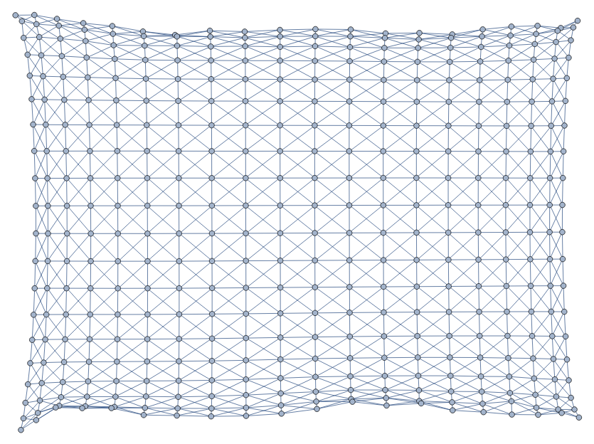
Before applying this code, let' s define a more realistic graph in which vertices are coupled to all nearest neighbors including diagonal directions. We also will define some initial conditions on our graph.

In[]:=

(*AdjHeatGridData=Import["/Users/jonlederman/Desktop/Wolfram Summer School/Project/Opus/Heatgrid/Adj.txt"];AdjHeatGridData=ImportString[AdjHeatGridData,"Table"][[1]];*)AdjHeatGridData=

If[

]

;AdjMatrixHeatGrid=ArrayReshape[AdjHeatGridData,{400,400}];(*HeatGridIC=Import["/Users/jonlederman/Desktop/Wolfram Summer School/Project/Opus/Heatgrid/C0.txt"];*)(*HeatGridIC=ImportString[HeatGridIC,"Table"][[1]];HeatGrid=AdjacencyGraph[AdjMatrixHeatGrid,VertexSize4.5];*)HeatGridIC=

;NormalizedHeatGridIC=NormalizeConditions[HeatGridIC];

In[]:=

anim=RunHeatKernelAnimation[HeatGrid,NormalizedHeatGridIC,0,5,0.2,500,7]

Out[]=

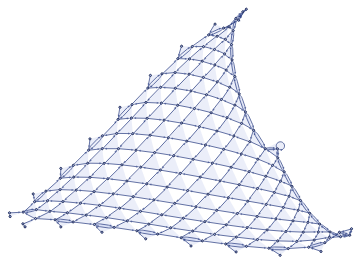
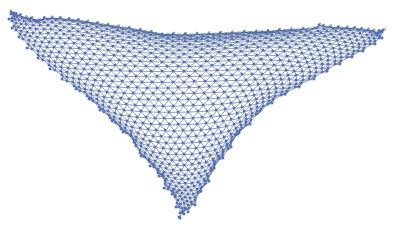
Next, we will apply this to one of the Wolfram Models. Specifically, we will look at 7714 from the Registry of Notable Universe Models. Before doing so, however, a fundamental question arises. Wolfram Model graphs are digraphs. However, the Laplacian matrix for digraphs is not well defined and in general will not be a symmetric positive-semidefinite matrix. One solution, which we adopt here, is to discard the directedness information and convert the graph to an undirected graph. Nonetheless, the validity of discarding the structure of the digraph is a question that warrants further consideration. In any case, we proceed with the approach of converting to an undirected graph.

In[]:=

(*WolframModelResourceFunctions*)WM=ResourceFunction["WolframModel"];HG2G=ResourceFunction["HypergraphToGraph"];Universe7714=WM[{{{1,2,2},{3,1,4}}{{2,5,2},{2,3,5},{4,5,5}}},{{1,1,1},{1,1,1}},750,"FinalState"];unig7714=HG2G[Universe7714,VertexSize4]

Out[]=

In[]:=

SetTemperatures[unig7714,ConstantArray[0,751]];

In[]:=

unig7714Delta=SetDeltaFunction[unig7714,200,4];ColorByInternalTemperature[unig7714Delta]

Out[]=

In[]:=

ic=GetTemperatures[unig7714Delta];anim7714=RunHeatKernelAnimation[unig7714,ic,0,5,0.2,500,7]

Out[]=

2. Weyl' s Law

Background

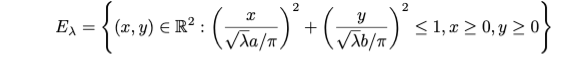
Weyl’s law has a rich history and diverse field of application. In general, it is a statement regarding the asymptotic growth of the eigenvalues of the Laplacian on bounded domains with DIrichlet or Neumann boundary conditions. The subject has roots in acoustics, specifically relating to the asymptotic behavior of the overtones of notes on instruments in a room, for example. In physics, the impetus for the development of Weyl’s law grew out of the black body radiation problem. Weyl' s law has been generalized to address non-Euclidean spaces such as d-dimensional manifolds with an associated Riemannian metric. In this case, the Laplacian must be replaced with the corresponding operator in these spaces, which is referred to as the Laplace-Beltrami operator. In the context of a manifold can be expressed as follows :

Here Ω⊂

d



is a bounded domain with an associated volume vol (Ω).

ω

d

is the volume of a unit ball in

d



and N(λ) is the number of eigenvalues of the Laplace-Beltrami operator less than λ.

A simple example illustrating Weyl’s law for a two-dimensional Dirichlet problem is derived by Matt Stevenson and proceeds as follows. We are interested in solving the following eigenvalue problem:

on the bounded domain Ω.

Take the boundary :

In two dimensions this becomes :

This equation can be solved using standard techniques such as separation of variables yielding the following separable solution :

The eigenvalues are :

Then, define an eigenvalue counting function :

This equation is suggestive of the coefficients of an ellipse equation. We can define an ellipse and the associated area in the first quadrant cut out by the ellipse by dividing by lambda and re-introducing the continuous variables x and y :

In[]:=

a=5;b=3;ContourPlot[(x/a)^2+(y/b)^21,{x,-5,5},{y,-3,3},AspectRatioAutomatic]

Out[]=

N(λ)issimplythenumberoflatticepointsinside

E

λ

For each eigenvalue pair, we can define a unit - area square :

The counting function can now be expressed as follows :

Exploration of Weyl’s Law WIth Respect to Wolfram Model Graphs Using The Laplacian Operator

As noted, a central issue concerns the appropriate analogue of the Laplace-Beltrami operator for d-dimensional manifolds in the context of graphs. This is an open question on the forefront of current research and will be discussed below in section 3. As a starting point, it will be instructive to attempt to naively apply the standard Laplacian operator to Wolfram Model graphs and examine whether the relationship holds in any form. Let us continue with Universe 7714. First, we will estimate it’s dimension as defined in the Wolfram Physics Project.

In[]:=

(*Firstwecreateauniverseandcalculatethegeodesicballsfromamedianvertex*)universe7714WM=WM[{{{1,2,2},{3,1,4}}{{2,5,2},{2,3,5},{4,5,5}}},{{1,1,1},{1,1,1}},2500,"FinalState"];universe77142500=HG2G[universe7714WM];medianVertex=Median@VertexList@universe77142500;geoBalls=NeighborhoodGraph[universe77142500,medianVertex,#]&/@Range[20];HighlightGraph[universe77142500,geoBalls]

Out[]=

In[]:=

(*ThefollowingcodeestimatesdimensionforagraphusinggeodesicballsandtheLogdifferencemetricasdefinedintheWolframPhysicsProject*)VOLS=Length@VertexList@geoBalls[[#]]&/@Range[Length[geoBalls]];dimensionList=N

(Log[VOLS[[#+1]]]-Log[VOLS[[#]]])

Log[#+1]-Log[#]

&@Range[Length[VOLS]-1];(*Hypergraphdimensionestimate*)HypergraphDimensionEstimateList[hg_]:=ResourceFunction["LogDifferences"][MeanAround/@Transpose[Values[ResourceFunction["HypergraphNeighborhoodVolumes"][hg,All,Automatic]]]];

It appears the dimension of this graph in the limit is 2. Now we will look at the eigenvalue spectrum on this graph using the standard Laplacian as it evolves up to a set number of iterations to determine whether any constant relationship can be established in the context of Weyl' s law.

In[]:=

(*CalculatesLaplacianmatricesforalistofgraphs*)laplacians=UnnormalizedLaplacian/@graphs;(*Calculateseigenvalueandeigenvectorforalistofgraphs*)EigenvalueList[graphs_]:=Sort/@Eigenvalues/@UnnormalizedLaplacian/@graphs;EigenvectorList[graphs_]:=Eigenvectors/@UnnormalizedLaplacian/@graphs;(*Calculatesnumberofeigenvaluesinalistoflistslessthanacertainnumber*)NumEigenvaluesLessThan[list_List,val_Integer]:=Length[Select[#1,LessThan[val]]]&/@list;NumEigenvaluesLessThanGraphs[graphs_,val_]:=NumEigenvaluesLessThan[EigenvalueList[graphs],val];(*Graphvolumecalculation*)Volumes[graphs_]:=VertexCount/@graphs;

Let us now evaluate this with respect to 2500 generations of our favorite universe 7714:

In[]:=

stateGenerations=WM[{{{1,2,2},{3,1,4}}{{2,5,2},{2,3,5},{4,5,5}}},{{1,1,1},{1,1,1}},100,"StatesList"];graphs=HG2G[#]&/@stateGenerations;minEigenvalueOverall=Min[Min/@EigenvalueList[graphs]];maxEigenvalueOverall=Max[Max/@EigenvalueList[graphs]];

In[]:=

maxEigenValueOverall

Out[]=

maxEigenValueOverall

We are now ready to define a simple function to test Weyl' s law using the naive definition of the Laplace - Beltrami operator as simply the Laplacian operator.

In[]:=

UnitBallVolume[graph_,v_]:=VertexCount[NeighborhoodGraph[graph,v,1]];WeylLeft[graphs_,lambda_,d_]:=NumEigenvaluesLessThanGraphs[graphs,lambda]/lambda^(d/2);WeylRight[graphs_,d_,vertex_,volume_]:=(N[2*Pi])^(-d)*UnitBallVolume[graph,vertex]*volume;

This completes all the computational machinery to evaluate whether Weyl' s law holds in this simple scenario and will be further investigated in future work.

3. The Laplace-Beltrami Operator

Background

The Laplace - Beltrami operator on a Riemannian manifold is defined formally as:

In[]:=

The functional form of this operator on a manifold can be derived by calculating the divergence and gradient operators for a manifold. The full derivation of this approach has been completed and will be provided in a future update of this article. Here is a brief sketch of the derivation. We seek to determine the generalization of the Laplacian operator on the manifold M with Riemannian metric g and tangent space

T

P

M

.

We first find the gradient of the function f on the manifold. Starting with the directional derivative as translated into the language of manifolds :

we ultimately find after some linear algebra :

Next we find the divergence of a vector field V on the manifold. The divergence operator maps the vector field to a scalar field in the tangent space. Starting with a relation that the the adjoint operator of the gradient is the negative of the divergence:

We can then integrate over all space :

After an integration by parts, we arrive at the divergence operator of a vector field on a manifold :

Combining the results for the gradient and divergence operators on the manifold, we arrive at the Laplace-Belatrami operator:

The Laplace - Beltrami Operator For Graphs

A fundamental question concerns what the appropriate analogue is for the Laplace - Beltrami operator on graphs. One potential approach with respect to the Wolfram Model graphs would be to define a discrete operator on graphs that takes into account the metric tensor, which may be spatially varying. Future work will investigate this approach.

4. Spectral Graph Theory

Spectral Graph Theory

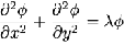
One fundamental question is the relationship between the Hausdorff dimension and spectral dimensions of a graph. The Hausdorff dimension is defined similarly to the notion of dimension as currently defined in the Wolfram Model using geodesic balls. The spectral dimension of a graph is defined as the return probability of a simple random walk to vertex v at time t.

In[]:=

where

p

G

(ω)

is a random walk. This spectral dimension definition may shed further light on Weyl’s law on graphs.

5. Conclusions And Future Work

We have implemented the mapping of the heat diffusion equation to a graph as a starting point for investigating the Laplacian operator in discrete domains. Next steps will involve evaluating whether any aspects of Weyl' s law can be observed using the simple Laplacian operator on graphs. In addition, a fundamental question that requires significant research is whether there exists a analog of the Laplace - Beltrami operator for graphs and how it may relate to the metric tensor as defined on Wolfram Model graphs.

References

◼

Arendt W, Nittka R, Peter W and Steiner F, Weyl’s Law: Spectral Properties of the Laplacian in Mathematics and Physics, Mathematical Analysis of Evolution, Information and Complexity (2009).

◼

Gorard, J,. Some Relativistic and Gravitational Properties of the Wolfram Model (2020).

◼

Ivrii, V., 100 Years of Weyl’s Law (2017).

◼

Reuter M., Wolter Franz-Enrich, Shenton M. and Niethammer Marc, Laplace-Beltrami Eigenvalues and Topological Features of Eigenfunctions for Statistical Shape Analysis (2009).

◼

Durhuus B., Hausdorff and Spectral DImensions of Infinite Random Graphs (2009).

◼

Stevenson, M. Weyl’s Law http://www-personal.umich.edu/~stevmatt/weyl_law.pdf (2014).

◼

Schmidt, F., The Laplace-Beltrami-Operator on Riemannian Manifolds.

◼

Wikipedia with respect to Weyl’s Law, Laplace-Beltrami Operator, Laplacian Matrix et al.

Complete project work

Heat Kernel

This notebook contains code for evaluating the heat kernel on graphs. Temperature on a graph is represented by the VertexWeigh of each vertex.

The following functions are for manipulating temperatures and associated coloring on a graph :

Sets temperatures for a graph by modifying the attributes of the graph provided.

In[]:=

Attributes[SetTemperatures]={HoldFirst};SetTemperatures[g_,temperatures_]:=AnnotationValue[g,VertexWeight]=temperatures

Sets temperatures for a graph by creating a new graph and returning the new graph.

In[]:=

SetTemperaturesNG[g_,tmps_]:=Module[{ng=g},AnnotationValue[{ng},VertexWeight]=tmps+1;ng]

Returns all temperatures for a graph :

In[]:=

GetTemperatures[g_]:=AnnotationValue[g,VertexWeight]

Colors a graph by temperature list:

In[]:=

ColorByTemperature[g_,temperatures_]:=HighlightGraph[g,MapThread[Style,{VertexList[g],Map[ColorData["TemperatureMap"],temperatures]}]]

Colors a graph by its internal temperatures (from already assigned VertexWeights) :

In[]:=

ColorByInternalTemperature[g_]:=ColorByTemperature[g,GetTemperatures[g]]

Normalizes temperatures on a graph between 0 and 1 :

In[]:=

Attributes[NormalizeTemperatures]={HoldFirst};NormalizeTemperatures[g_]:=SetTemperatures[g,N[#/Max[#]]]&@GetTemperatures[g]

The following code implements the heat kernel dynamics :

UnnormalizedLaplacian returns the unnormalized Laplacian of the associated undirected graph.
GraphSpectrum returns the eigenvalues and eigenfunctions of the graph input object as an associative array.

In[]:=

UnnormalizedLaplacian[g_]:=N@(DiagonalMatrix[VertexOutDegree[#]]-AdjacencyMatrix[#])&@UndirectedGraph[g]

In[]:=

GraphSpectrum[g_]:=<|"eigenvalues"->Eigenvalues[#],"eigenvectors"->Eigenvectors[#]|>&@UnnormalizedLaplacian[g]

The following functions project onto the eigenspace and back to the temperature space respectively.

In[]:=

EigenSpaceProject[ic_,eigenvectors_]:=eigenvectors.ic

In[]:=

VertexSpaceProject[vector_,eigenvectors_]:=Transpose[eigenvectors].vector

The following function performs temporal evolution in the eigenspace.

In[]:=

EigenSpaceAdvance[spectrum_,coordinates_,t_]:=Exp[-t*spectrum["eigenvalues"]]*coordinates

The following function performs temporal evolution in temperature space returning the advanced temperature vector from initial conditions.

In[]:=

TemperatureSpaceAdvance[spectrum_,ic_,t_]:=VertexSpaceProject[EigenSpaceAdvance[spectrum,EigenSpaceProject[ic,#],t],#]&@spectrum["eigenvectors"]

The following function temporally advances the heat distribution on a graph by modifying the provided graph object.

In[]:=

Attributes[TimePropagate]={HoldFirst};TimePropagate[g_,t_]:=SetTemperatures[g,TemperatureSpaceAdvance[GraphSpectrum[g],GetTemperatures[g],t]]

In[]:=

The following function generates a list of temperature space vectors corresponding to a range of times as specified by a start, stop and increment using initial conditions bsed on the current graph temperatures.

In[]:=

TemperatureSpaceAdvanceInterval[spectrum_,ic_,start_,stop_,increment_]:=VertexSpaceProject[EigenSpaceAdvanceRange[start,stop,increment,#[[2]],EigenSpaceProject[ic,#[[1]]]],#[[1]]]&@{spectrum["eigenvectors"],spectrum["eigenvalues"]}

The following function generates a range of advancements in eigenspace for a set of times from start to stop with increment.

In[]:=

EigenSpaceMakeRange[start_,stop_,increment_,eigenvalues_]:=Exp[-#*eigenvalues]&/@Range[start,stop,increment]

The following function advances coordinates in eigenspace over a range of times using EigenSpaceMakeRange

EigenSpaceAdvanceRange[start_,stop_,increment_,eigenvalues_,coordinates_]:=Transpose[EigenSpaceMakeRange[start,stop,increment,eigenvalues]]*coordinates

In[]:=

TemperatureSpaceAdvance[GraphSpectrum[gridSmall],Range[1,9],0.6]

Out[]=

{2.80475,3.35357,3.90238,4.45119,5.,5.54881,6.09762,6.64643,7.19525}

In[]:=

VertexSpaceProject[EigenSpaceAdvanceRange[0.5,0.6,0.1,GraphSpectrum[gridSmall]["eigenvalues"],EigenSpaceProject[Range[1,9],GraphSpectrum[gridSmall]["eigenvectors"]]],GraphSpectrum[gridSmall]["eigenvectors"]]

Out[]=

{{2.57388,2.80475},{3.18041,3.35357},{3.78694,3.90238},{4.39347,4.45119},{5.,5.},{5.60653,5.54881},{6.21306,6.09762},{6.81959,6.64643},{7.42612,7.19525}}

In[]:=

GetTemperatures[gridGraph]

Out[]=

{0.,0.010101,0.020202,0.030303,0.040404,0.0505051,0.0606061,0.0707071,0.0808081,0.0909091,0.10101,0.111111,0.121212,0.131313,0.141414,0.151515,0.161616,0.171717,0.181818,0.191919,0.20202,0.212121,0.222222,0.232323,0.242424,0.252525,0.262626,0.272727,0.282828,0.292929,0.30303,0.313131,0.323232,0.333333,0.343434,0.353535,0.363636,0.373737,0.383838,0.393939,0.40404,0.414141,0.424242,0.434343,0.444444,0.454545,0.464646,0.474747,0.484848,0.494949,0.505051,0.515152,0.525253,0.535354,0.545455,0.555556,0.565657,0.575758,0.585859,0.59596,0.606061,0.616162,0.626263,0.636364,0.646465,0.656566,0.666667,0.676768,0.686869,0.69697,0.707071,0.717172,0.727273,0.737374,0.747475,0.757576,0.767677,0.777778,0.787879,0.79798,0.808081,0.818182,0.828283,0.838384,0.848485,0.858586,0.868687,0.878788,0.888889,0.89899,0.909091,0.919192,0.929293,0.939394,0.949495,0.959596,0.969697,0.979798,0.989899,1.}

In[]:=

VertexSpaceProject[EigenSpaceProject[GetTemperatures[gridGraph],GraphSpectrum[gridGraph]["eigenvectors"]],GraphSpectrum[gridGraph]["eigenvectors"]]

Out[]=

{0.333565,0.335047,0.337865,0.341743,0.3463,0.351091,0.355649,0.359526,0.362344,0.363826,0.348383,0.349865,0.352683,0.356561,0.361118,0.36591,0.370467,0.374344,0.377162,0.378644,0.376563,0.378045,0.380863,0.38474,0.389298,0.394089,0.398647,0.402524,0.405342,0.406824,0.415339,0.41682,0.419638,0.423516,0.428073,0.432865,0.437422,0.4413,0.444118,0.445599,0.460912,0.462394,0.465212,0.469089,0.473647,0.478438,0.482996,0.486873,0.489691,0.491173,0.508827,0.510309,0.513127,0.517004,0.521562,0.526353,0.530911,0.534788,0.537606,0.539088,0.554401,0.555882,0.5587,0.562578,0.567135,0.571927,0.576484,0.580362,0.58318,0.584661,0.593176,0.594658,0.597476,0.601353,0.605911,0.610702,0.61526,0.619137,0.621955,0.623437,0.621356,0.622838,0.625656,0.629533,0.63409,0.638882,0.643439,0.647317,0.650135,0.651617,0.636174,0.637656,0.640474,0.644351,0.648909,0.6537,0.658257,0.662135,0.664953,0.666435}

In[]:=

GetTemperatures[gridGraph]

Out[]=

Automatic

In[]:=

Transpose[EigenSpaceAdvanceRange[0.5,0.6,0.1,GraphSpectrum[gridSmall]["eigenvalues"],EigenSpaceProject[GetTemperatures[gridSmall],GraphSpectrum[gridSmall]["eigenvectors"]]]]

Out[]=

{{-1.10549×

-17

10

,4.50757×

-17

10

,1.7279×

-16

10

,1.11476×

-16

10

,2.10566×

-16

10

,6.94328×

-16

10

,-0.233454,0.466908,-1.66667},{-6.06709×

-18

10

,3.02151×

-17

10

,1.15825×

-16

10

,8.25834×

-17

10

,1.55991×

-16

10

,5.68468×

-16

10

,-0.211238,0.422475,-1.66667}}

In[]:=

TemperatureSpaceAdvanceInterval[GraphSpectrum[gridSmall],Range[1,9],0.5,0.6,0.1]

Out[]=

{{2.57388,2.80475},{3.18041,3.35357},{3.78694,3.90238},{4.39347,4.45119},{5.,5.},{5.60653,5.54881},{6.21306,6.09762},{6.81959,6.64643},{7.42612,7.19525}}

In[]:=

EigenSpaceAdvance[GraphSpectrum[gridGraph],EigenSpaceProject[GetTemperatures[gridGraph],GraphSpectrum[gridGraph]["eigenvalues"]],0.5]

Out[]=

{3.21288,3.70323,3.70323,4.26843,4.6202,4.6202,5.32534,5.32534,6.1056,6.1056,6.64396,7.03745,7.03745,8.31635,8.31635,8.78001,8.78001,9.5856,9.5856,11.3276,11.3276,11.6028,11.9591,11.9591,13.0564,13.0564,14.9694,14.9694,15.804,15.804,16.2893,16.2893,17.2541,17.2541,18.676,18.676,21.5264,21.5264,21.5264,21.5264,21.5264,21.5264,21.5264,21.5264,21.5264,22.6062,22.6062,24.8118,24.8118,26.0564,26.0564,26.8566,26.8566,28.4471,28.4471,29.3208,29.3208,30.9555,30.9555,32.5083,32.5083,35.491,35.491,38.7474,38.7474,39.9374,40.9077,40.9077,42.9597,42.9597,48.3418,48.3418,52.7773,52.7773,55.7198,55.7198,58.5148,58.5148,65.8457,65.8457,69.7453,75.8952,75.8952,79.7021,79.7021,87.0151,87.0151,100.296,100.296,105.326,105.326,108.561,125.13,125.13,131.407,131.407,144.228,151.462,151.462,159.06}

In[]:=

Dimensions[%]

Out[]=

{2,100}

In[]:=

EigenSpaceAdvance[GraphSpectrum[gridGraph],GetTemperatures[gridGraph],0.6]

Out[]=

{0.00308732,0.00367731,0.00370824,0.00444783,0.00495648,0.00502506,0.00603624,0.00610205,0.00724641,0.00727605,0.00771078,0.00829711,0.00836394,0.0103319,0.010464,0.0113161,0.011457,0.012863,0.0129598,0.0158973,0.0158099,0.016336,0.0170661,0.0172399,0.019382,0.0196205,0.0233863,0.0236138,0.0253787,0.0254715,0.0269659,0.0270621,0.0291926,0.0294623,0.0327482,0.0331147,0.039682,0.0400338,0.0402894,0.0404239,0.041813,0.0419474,0.0422031,0.0425548,0.0429683,0.0460284,0.0464669,0.0523761,0.0526793,0.056035,0.058049,0.0603701,0.0607035,0.0655343,0.0661119,0.0691856,0.0697846,0.0750231,0.0754184,0.080201,0.0824791,0.0918867,0.0923525,0.103324,0.104161,0.108924,0.113001,0.113761,0.121228,0.121536,0.142069,0.142424,0.158996,0.160027,0.172087,0.173448,0.185313,0.186481,0.215834,0.216348,0.231039,0.256306,0.257466,0.274733,0.276722,0.309786,0.311996,0.372205,0.373826,0.397343,0.387926,0.403203,0.480245,0.483152,0.516003,0.519813,0.585304,0.624366,0.627024,0.666435}

In[]:=

EigenSpaceAdvance[GraphSpectrum[gridGraph],ConstantArray[1,100],0.6]

Out[]=

{0.00925552,0.0109755,0.0109755,0.0130152,0.0143127,0.0143127,0.0169725,0.0169725,0.0199987,0.0199987,0.022133,0.0237152,0.0237152,0.0289766,0.0289766,0.0309259,0.0309259,0.0343614,0.0343614,0.0419848,0.0419848,0.0432118,0.0448092,0.0448092,0.0497871,0.0497871,0.0586642,0.0586642,0.0626106,0.0626106,0.064925,0.064925,0.0695661,0.0695661,0.0765013,0.0765013,0.090718,0.090718,0.090718,0.090718,0.090718,0.090718,0.090718,0.090718,0.090718,0.0962056,0.0962056,0.107577,0.107577,0.114084,0.114084,0.118301,0.118301,0.126758,0.126758,0.131443,0.131443,0.140286,0.140286,0.148772,0.148772,0.165299,0.165299,0.183662,0.183662,0.190451,0.196017,0.196017,0.207875,0.207875,0.239505,0.239505,0.266112,0.266112,0.284014,0.284014,0.301194,0.301194,0.347025,0.347025,0.371831,0.411514,0.411514,0.436407,0.436407,0.484888,0.484888,0.574997,0.574997,0.60978,0.60978,0.63232,0.749828,0.749828,0.795186,0.795186,0.889172,0.942959,0.942959,1.}

In[]:=

Dimensions[%]

Out[]=

{100}

In[]:=

Dimensions[a]

The next set of code tests our graph temperature code.

In[]:=

gridGraph=GridGraph[{10,10}]

Out[]=

In[]:=

SetTemperatures[gridGraph,Range[0,99]]

Out[]=

{0,1,2,3,4,5,6,7,8,9,10,11,12,13,14,15,16,17,18,19,20,21,22,23,24,25,26,27,28,29,30,31,32,33,34,35,36,37,38,39,40,41,42,43,44,45,46,47,48,49,50,51,52,53,54,55,56,57,58,59,60,61,62,63,64,65,66,67,68,69,70,71,72,73,74,75,76,77,78,79,80,81,82,83,84,85,86,87,88,89,90,91,92,93,94,95,96,97,98,99}

In[]:=

{0,1,2,3,4,5,6,7,8,9,10,11,12,13,14,15,16,17,18,19,20,21,22,23,24,25,26,27,28,29,30,31,32,33,34,35,36,37,38,39,40,41,42,43,44,45,46,47,48,49,50,51,52,53,54,55,56,57,58,59,60,61,62,63,64,65,66,67,68,69,70,71,72,73,74,75,76,77,78,79,80,81,82,83,84,85,86,87,88,89,90,91,92,93,94,95,96,97,98,99}

Out[]=

{0,1,2,3,4,5,6,7,8,9,10,11,12,13,14,15,16,17,18,19,20,21,22,23,24,25,26,27,28,29,30,31,32,33,34,35,36,37,38,39,40,41,42,43,44,45,46,47,48,49,50,51,52,53,54,55,56,57,58,59,60,61,62,63,64,65,66,67,68,69,70,71,72,73,74,75,76,77,78,79,80,81,82,83,84,85,86,87,88,89,90,91,92,93,94,95,96,97,98,99}

In[]:=

NormalizeTemperatures[gridGraph];ColorByInternalTemperature[gridGraph]

Out[]=

In[]:=

d

Out[]=

d

In[]:=

UnnormalizedLaplacian[gridGraph];

In[]:=

nl=UnnormalizedLaplacian[gridGraph];Dimensions[nl]Eigenvectors[nl]completeGraph=CompleteGraph[10]

Out[]=

{100,100}

Out[]=

{{0.00489435,-0.014204,0.0221232,-0.0278768,0.0309017,-0.0309017,0.0278768,-0.0221232,0.014204,-0.00489435,-0.014204,0.0412215,

⋯77⋯

,-0.014204,-0.00489435,0.014204,-0.0221232,0.0278768,-0.0309017,0.0309017,-0.0278768,0.0221232,-0.014204,0.00489435},

⋯98⋯

,{

⋯1⋯

}}

large output

show less

show all

set size limit...

Out[]=

In[]:=

SetTemperatures[gridGraph,Range[0,99]]

Out[]=

{0,1,2,3,4,5,6,7,8,9,10,11,12,13,14,15,16,17,18,19,20,21,22,23,24,25,26,27,28,29,30,31,32,33,34,35,36,37,38,39,40,41,42,43,44,45,46,47,48,49,50,51,52,53,54,55,56,57,58,59,60,61,62,63,64,65,66,67,68,69,70,71,72,73,74,75,76,77,78,79,80,81,82,83,84,85,86,87,88,89,90,91,92,93,94,95,96,97,98,99}

In[]:=

NormalizeTemperatures[gridGraph]

Out[]=

{0.,0.010101,0.020202,0.030303,0.040404,0.0505051,0.0606061,0.0707071,0.0808081,0.0909091,0.10101,0.111111,0.121212,0.131313,0.141414,0.151515,0.161616,0.171717,0.181818,0.191919,0.20202,0.212121,0.222222,0.232323,0.242424,0.252525,0.262626,0.272727,0.282828,0.292929,0.30303,0.313131,0.323232,0.333333,0.343434,0.353535,0.363636,0.373737,0.383838,0.393939,0.40404,0.414141,0.424242,0.434343,0.444444,0.454545,0.464646,0.474747,0.484848,0.494949,0.505051,0.515152,0.525253,0.535354,0.545455,0.555556,0.565657,0.575758,0.585859,0.59596,0.606061,0.616162,0.626263,0.636364,0.646465,0.656566,0.666667,0.676768,0.686869,0.69697,0.707071,0.717172,0.727273,0.737374,0.747475,0.757576,0.767677,0.777778,0.787879,0.79798,0.808081,0.818182,0.828283,0.838384,0.848485,0.858586,0.868687,0.878788,0.888889,0.89899,0.909091,0.919192,0.929293,0.939394,0.949495,0.959596,0.969697,0.979798,0.989899,1.}

In[]:=

TimePropagate[gridGraph,10]

Out[]=

{0.333565,0.335047,0.337865,0.341743,0.3463,0.351091,0.355649,0.359526,0.362344,0.363826,0.348383,0.349865,0.352683,0.356561,0.361118,0.36591,0.370467,0.374344,0.377162,0.378644,0.376563,0.378045,0.380863,0.38474,0.389298,0.394089,0.398647,0.402524,0.405342,0.406824,0.415339,0.41682,0.419638,0.423516,0.428073,0.432865,0.437422,0.4413,0.444118,0.445599,0.460912,0.462394,0.465212,0.469089,0.473647,0.478438,0.482996,0.486873,0.489691,0.491173,0.508827,0.510309,0.513127,0.517004,0.521562,0.526353,0.530911,0.534788,0.537606,0.539088,0.554401,0.555882,0.5587,0.562578,0.567135,0.571927,0.576484,0.580362,0.58318,0.584661,0.593176,0.594658,0.597476,0.601353,0.605911,0.610702,0.61526,0.619137,0.621955,0.623437,0.621356,0.622838,0.625656,0.629533,0.63409,0.638882,0.643439,0.647317,0.650135,0.651617,0.636174,0.637656,0.640474,0.644351,0.648909,0.6537,0.658257,0.662135,0.664953,0.666435}

In[]:=

ColorByInternalTemperature[gridGraph]

Out[]=

In[]:=

ColorByInternalTemperature[gridGraph]

Out[]=

In[]:=

GetTemperatures[gridGraph]

Out[]=

{0.333565,0.335047,0.337865,0.341743,0.3463,0.351091,0.355649,0.359526,0.362344,0.363826,0.348383,0.349865,0.352683,0.356561,0.361118,0.36591,0.370467,0.374344,0.377162,0.378644,0.376563,0.378045,0.380863,0.38474,0.389298,0.394089,0.398647,0.402524,0.405342,0.406824,0.415339,0.41682,0.419638,0.423516,0.428073,0.432865,0.437422,0.4413,0.444118,0.445599,0.460912,0.462394,0.465212,0.469089,0.473647,0.478438,0.482996,0.486873,0.489691,0.491173,0.508827,0.510309,0.513127,0.517004,0.521562,0.526353,0.530911,0.534788,0.537606,0.539088,0.554401,0.555882,0.5587,0.562578,0.567135,0.571927,0.576484,0.580362,0.58318,0.584661,0.593176,0.594658,0.597476,0.601353,0.605911,0.610702,0.61526,0.619137,0.621955,0.623437,0.621356,0.622838,0.625656,0.629533,0.63409,0.638882,0.643439,0.647317,0.650135,0.651617,0.636174,0.637656,0.640474,0.644351,0.648909,0.6537,0.658257,0.662135,0.664953,0.666435}

In[]:=

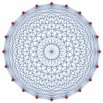
SetTemperatures[completeGraph,Range[0.1,1,0.1]]

Out[]=

{0.1,0.2,0.3,0.4,0.5,0.6,0.7,0.8,0.9,1.}

In[]:=

ColorByTemperature[completeGraph,Range[0,0.9,0.1]]

Out[]=

In[]:=

ColorByInternalTemperature[completeGraph]

Out[]=

In[]:=

AnnotationValue[{completeGraph},VertexWeight]=Range[10]

Out[]=

{1,2,3,4,5,6,7,8,9,10}

In[]:=

AnnotationValue[{completeGraph,1},VertexWeight]=2

In[]:=

GetTemperatures[completeGraph]

Out[]=

{2,2,3,4,5,6,7,8,9,10}

In[]:=

SetTemperatures[completeGraph,Range[10,19]]

Out[]=

{10,11,12,13,14,15,16,17,18,19}

In[]:=

GetTemperatures[completeGraph]

Out[]=

{10,11,12,13,14,15,16,17,18,19}

In[]:=

NormalizeTemperatures[completeGraph]

Out[]=

{0.526316,0.578947,0.631579,0.684211,0.736842,0.789474,0.842105,0.894737,0.947368,1.}

In[]:=

GetTemperatures[completeGraph]

Out[]=

{0.526316,0.578947,0.631579,0.684211,0.736842,0.789474,0.842105,0.894737,0.947368,1.}

In[]:=

FullForm[completeGraph]

Out[]//FullForm=

Graph[List[1,2,3,4,5,6,7,8,9,10],List[Null,SparseArray[Automatic,List[10,10],0,List[1,List[List[0,9,18,27,36,45,54,63,72,81,90],List[List[2],List[3],List[4],List[5],List[6],List[7],List[8],List[9],List[10],List[1],List[3],List[4],List[5],List[6],List[7],List[8],List[9],List[10],List[1],List[2],List[4],List[5],List[6],List[7],List[8],List[9],List[10],List[1],List[2],List[3],List[5],List[6],List[7],List[8],List[9],List[10],List[1],List[2],List[3],List[4],List[6],List[7],List[8],List[9],List[10],List[1],List[2],List[3],List[4],List[5],List[7],List[8],List[9],List[10],List[1],List[2],List[3],List[4],List[5],List[6],List[8],List[9],List[10],List[1],List[2],List[3],List[4],List[5],List[6],List[7],List[9],List[10],List[1],List[2],List[3],List[4],List[5],List[6],List[7],List[8],List[10],List[1],List[2],List[3],List[4],List[5],List[6],List[7],List[8],List[9]]],Pattern]]],List[Rule[GraphLayout,List["CircularEmbedding",Rule["OptimalOrder",False]]],Rule[VertexWeight,List[0.5263157894736842`,0.5789473684210527`,0.631578947368421`,0.6842105263157895`,0.7368421052631579`,0.7894736842105263`,0.8421052631578947`,0.8947368421052632`,0.9473684210526315`,1.`]]]]

In[]:=

AnnotationValue[{completeGraph,1},VertexWeight]

Out[]=

0.526316

In[]:=

pre={<computation>};ListAnimate[pre]

In[]:=

gridSmall=GridGraph[{3,3}]

Out[]=

In[]:=

SetTemperatures[gridSmall,Range[1,9]]

Out[]=

{1,2,3,4,5,6,7,8,9}

In[]:=

GetTemperatures[gridSmall]

Out[]=

{1,2,3}

In[]:=

NormalizeTemperatures[gridSmall]

Out[]=

{0.111111,0.222222,0.333333,0.444444,0.555556,0.666667,0.777778,0.888889,1.}

In[]:=

lap=N[UnnormalizedLaplacian[gridSmall]]

Out[]=

{{2.,-1.,0.,-1.,0.,0.,0.,0.,0.},{-1.,3.,-1.,0.,-1.,0.,0.,0.,0.},{0.,-1.,2.,0.,0.,-1.,0.,0.,0.},{-1.,0.,0.,3.,-1.,0.,-1.,0.,0.},{0.,-1.,0.,-1.,4.,-1.,0.,-1.,0.},{0.,0.,-1.,0.,-1.,3.,0.,0.,-1.},{0.,0.,0.,-1.,0.,0.,2.,-1.,0.},{0.,0.,0.,0.,-1.,0.,-1.,3.,-1.},{0.,0.,0.,0.,0.,-1.,0.,-1.,2.}}

In[]:=

eigvectors=Transpose[GraphSpectrum[gridSmall]["eigenvectors"]]//MatrixForm

Out[]//MatrixForm=

-0.166667	1.39278× -16 10	-0.408248	5.24441× -16 10	0.333333	0.5	5.12338× -16 10	-0.57735	-0.333333
0.333333	0.408248	0.408248	-0.5	-0.166667	-1.25076× -15 10	0.288675	-0.288675	-0.333333
-0.166667	-0.408248	-2.42266× -16 10	3.72043× -16 10	0.333333	-0.5	0.57735	5.50592× -16 10	-0.333333
0.333333	-0.408248	0.408248	0.5	-0.166667	-1.16461× -15 10	-0.288675	-0.288675	-0.333333
-0.666667	-2.802× -16 10	-2.29491× -15 10	-1.66492× -16 10	-0.666667	1.2785× -16 10	4.13609× -16 10	3.12004× -16 10	-0.333333
0.333333	0.408248	-0.408248	0.5	-0.166667	1.37033× -15 10	0.288675	0.288675	-0.333333
-0.166667	0.408248	7.6891× -17 10	5.59715× -16 10	0.333333	-0.5	-0.57735	1.21435× -17 10	-0.333333
0.333333	-0.408248	-0.408248	-0.5	-0.166667	1.22019× -15 10	-0.288675	0.288675	-0.333333
-0.166667	0.	0.408248	0.	0.333333	0.5	0.	0.57735	-0.333333

In[]:=

eigenvalues=GraphSpectrum[gridSmall]["eigenvalues"]

Out[]=

{6.,4.,4.,3.,3.,2.,1.,1.,6.76542×

-16

10

}

In[]:=

EigenSpaceProject[Range[1,9],GraphSpectrum[gridSmall]["eigenvectors"]]

Out[]=

{-1.55431×

-15

10

,3.10862×

-15

10

,1.11022×

-14

10

,3.55271×

-15

10

,7.54952×

-15

10

,1.59872×

-14

10

,-3.4641,6.9282,-15.}

In[]:=

GraphSpectrum[gridSmall]["eigenvalues"]

Out[]=

{6.,4.,4.,3.,3.,2.,1.,1.,6.76542×

-16

10

}

In[]:=

a=AdjacencyMatrix[dg]//MatrixForm

Out[]//MatrixForm=

0	1	0
0	0	1
1	0	0

In[]:=

Eigenvalues[ul]//MatrixForm

Out[]//MatrixForm=

3

1

0

In[]:=

Eigenvalues[UnnormalizedLaplacian[dg]]

Out[]=



3.54

…

,

2.79

…

,1+

2

,

2.30

…

,

-1.16

…

,

0.775

…

,

-0.581

…

,1-

2

,

0.337

…



In[]:=

Eigenvectors[UnnormalizedLaplacian[dg]]

Out[]=



1

14

-13+16

3.54

…

-8

2

3.54

…

+13

3

3.54

…

+16

4

3.54

…

-16

5

3.54

…

+3

6

3.54

…

,

1

28

-57+82

3.54

…

+64

2

3.54

…

-83

3

3.54

…

-2

4

3.54

…

+16

5

3.54

…

-3

6

3.54

…

,

1

28

-19+74

3.54

…

-44

2

3.54

…

-65

3

3.54

…

+46

4

3.54

…

-4

5

3.54

…

-

6

3.54

…

,

1

4

7+

⋯7⋯

+

6

3.54

…

,

1

7

(

⋯1⋯

),

1

28

(

⋯1⋯

),1-

3.54

…

,

1

4

-7-14

3.54

…

+36

2

3.54

…

-

3

3.54

…

-18

4

3.54

…

+8

5

3.54

…

-

6

3.54

…

,1,

⋯7⋯

,{

⋯1⋯

}

large output

show less

show all

set size limit...

In[]:=

{1,2,3}//MatrixForm

Out[]//MatrixForm=

1

2

3

In[]:=

UnnormalizedLaplacian[g_]:=N@(DiagonalMatrix[VertexOutDegree[#]]-AdjacencyMatrix[#])&@UndirectedGraph[g]

In[]:=

Unnormalizedlaplacian[dg]//MatrixForm

Out[]//MatrixForm=

1	-1	0	0	0	0
-1	3	-1	0	0	-1
0	-1	4	-1	-1	-1
0	0	-1	2	-1	0
0	0	-1	-1	3	-1
0	-1	-1	0	-1	3

In[]:=

DigraphSpectrum[g_]:=<|"eigenvalues"->Eigenvalues[#],"eigenvectors"->Eigenvectors[#]|>&@Unnormalizedlaplacian[g]

In[]:=

DigraphSpectrum[dg]

Out[]=

In[]:=

N[EigenspaceAdvance[DigraphSpectrum[dg],1]]

Out[]=

{{-0.00819429,0.0337464,-0.0692764,0.0148887,0.0228494,0.00598629},{0.00157391,-0.00558638,-0.0034926,0.00423499,-0.00730392,0.010574},{0.0390194,-0.0962183,-0.0254349,-0.0557068,0.107096,0.0312446},{-0.0724067,0.0822007,0.0252752,-0.14803,-0.00525218,0.118214},{-3.08843,-0.830214,0.723486,1.51502,1.1988,0.481338},{1.,1.,1.,1.,1.,1.}}

In[]:=

EigenspaceAdvance[spectrum_,coordinates_,t_]:=Exp[-t*spectrum["eigenvalues"]]*coordinates

In[]:=

EigenspaceProject[ic,eigenvectors]:=eigenvectors.icVertexspaceProject[vectors,eigenvectors]:=Transpose[eigenvectors].vectorsTimeEvolve[spectrum_,ic_,t_]:=VertexspaceProject[EigenspaceAdvance[spectrum,EigenspaceProject[ic,#],t],#]&@spectrum["eigenvectors"]

In[]:=

DigraphSpectrum[dg]["eigenvalues"]

Out[]=



5.12

…

,

4.55

…

,

3.47

…

,

2.14

…

,

0.731

…

,0

In[]:=

N[MatrixExp[{{1,0},{0,2}}]]

Out[]=

{{2.71828,0.},{0.,7.38906}}

In[]:=

Graph[{1,2,Style[3,Red]},{12,23,Style[31,Blue]}]

Out[]=

In[]:=

ag=Graph[{12,23,31},VertexWeight{2,3,4}]AnnotationValue[{ag,1},VertexWeight]=5

Out[]=

5

In[]:=

AnnotationValue[ag,VertexWeight]

Out[]=

{5,3,4}

In[]:=

AnnotationValue[ag,VertexWeight]

Out[]=

{2,3,4}

In[]:=

VertexList[ag1]

Out[]=

{2,3,1}

In[]:=

ag1=Graph[{23,12,31},VertexWeight{2,3,4}]

Out[]=

In[]:=

TableForm[Normal[AdjacencyMatrix[ag1]],TableHeadings{VertexList[ag1],VertexList[ag1]}]

Out[]//TableForm=

	2	3	1
2	0	1	1
3	1	0	1
1	1	1	0

In[]:=

g=CycleGraph[5,VertexWeightTable[0,5],VertexLabels"VertexWeight"];Manipulate[Module[{v=i},AnnotationValue[g,VertexWeight]=Table[0,5];AnnotationValue[{g,v},VertexWeight]=1;MapThread[(AnnotationValue[{g,#1},VertexStyle]=If[#2>0,Red,Blue])&,{VertexList[g],AnnotationValue[g,VertexWeight]}];g],{i,Range[5]},TrackedSymbols{i}]

In[]:=

DigraphSpectrum[g_]:=<|"eigenvalues"->Eigenvalues[#],"eigenvectors"->Eigenvectors[#]|>&@Unnormalizedlaplacian[g]

In[]:=

DigraphSpectrum[dg]

Out[]=

In[]:=

N[EigenspaceAdvance[DigraphSpectrum[dg],1]]

Out[]=

{{-0.00819429,0.0337464,-0.0692764,0.0148887,0.0228494,0.00598629},{0.00157391,-0.00558638,-0.0034926,0.00423499,-0.00730392,0.010574},{0.0390194,-0.0962183,-0.0254349,-0.0557068,0.107096,0.0312446},{-0.0724067,0.0822007,0.0252752,-0.14803,-0.00525218,0.118214},{-3.08843,-0.830214,0.723486,1.51502,1.1988,0.481338},{1.,1.,1.,1.,1.,1.}}

In[]:=

EigenspaceAdvance[spectrum_,coordinates_,t_]:=Exp[-t*spectrum["eigenvalues"]]*coordinates

In[]:=

SetOptions[EvaluationNotebook[],BackgroundWhite]

In[]:=

EigenspaceProject[ic,eigenvectors]:=eigenvectors.icVertexspaceProject[vectors,eigenvectors]:=Transpose[eigenvectors].vectorsTimeEvolve[spectrum_,ic_,t_]:=VertexspaceProject[EigenspaceAdvance[spectrum,EigenspaceProject[ic,#],t],#]&@spectrum["eigenvectors"]

In[]:=

DigraphSpectrum[dg]["eigenvalues"]

Out[]=



5.12

…

,

4.55

…

,

3.47

…

,

2.14

…

,

0.731

…

,0

In[]:=

Graph[{1,2,Style[3,Red]},{12,23,Style[31,Blue]}]

Out[]=

In[]:=

ag=Graph[{12,23,31},VertexWeight{2,3,4}]AnnotationValue[{ag,1},VertexWeight]=5

Out[]=

5

In[]:=

AnnotationValue[ag,VertexWeight]

In[]:=

AnnotationValue[ag,VertexWeight]

Out[]=

{2,3,4}

In[]:=

VertexList[ag1]

Out[]=

{2,3,1}

In[]:=

ag1=Graph[{23,12,31},VertexWeight{2,3,4}]

Out[]=

In[]:=

TableForm[Normal[AdjacencyMatrix[ag1]],TableHeadings{VertexList[ag1],VertexList[ag1]}]

Out[]//TableForm=

	2	3	1
2	0	1	1
3	1	0	1
1	1	1	0

In[]:=

g=CycleGraph[5,VertexWeightTable[0,5],VertexLabels"VertexWeight"];Manipulate[Module[{v=i},AnnotationValue[g,VertexWeight]=Table[0,5];AnnotationValue[{g,v},VertexWeight]=1;MapThread[(AnnotationValue[{g,#1},VertexStyle]=If[#2>0,Red,Blue])&,{VertexList[g],AnnotationValue[g,VertexWeight]}];g],{i,Range[5]},TrackedSymbols{i}]

In[]:=

Exp[-t*{lambda1,lambda2,lamba3}*{1,2,3}]*{{1,2,3},{4,5,6},{7,8,9}}

Out[]=



-lambda1t



,2

-lambda1t



,3

-lambda1t



,4

-2lambda2t



,5

-2lambda2t



,6

-2lambda2t



,7

-3lamba3t



,8

-3lamba3t



,9

-3lamba3t





In[]:=

Length[AdjTestList]

Out[]=

160000

In[]:=

Dimensions[AdjTestMatrix]

Out[]=

{400,400}

In[]:=

AdjTestGraph=AdjacencyGraph[AdjTestMatrix]

Out[]=

In[]:=

EdgeCount[AdjTestGraph]

Out[]=

1482

In[]:=

VertexCount[AdjTestGraph]

Out[]=

400

In[]:=

FindClique[AdjTestGraph,Infinity,All];

In[]:=

HG2G=ResourceFunction["HypergraphToGraph"]

Out[]=

[◼]	HypergraphToGraph

In[]:=

[◼]	HypergraphToGraph

In[]:=

ResourceFunction["HypergraphToGraph"][{{1,3,2},{2,1,3}}]

Out[]=

In[]:=

{{x,y,y},{z,x,u}}{{y,v,y},{y,z,v},{u,v,v}}

Out[]=

{{x,y,y},{z,x,u}}{{y,v,y},{y,z,v},{u,v,v}}

In[]:=

[◼]	WolframModel

[{{{1,1,2}}{{1,1,2},{1,2,3}}},{{1,1,1}},6,"StatesPlotsList"]

Out[]=



,



In[]:=

WolframModel[]["FinalStatePlot"]

Out[]=

WolframModel[][FinalStatePlot]

In[]:=

[◼]	WolframModel

[{{{1,1,2}}{{1,1,2},{1,2,3}}},{{1,1,1}},<|"MaxEvents"6|>,"EventsStatesPlotsList"]

In[]:=

{vertexCountList,edgeCountList}=

[◼]	WolframModel

[{{{1,1,2}}{{1,1,2},{1,2,3}}},{{1,1,1}},199,{"VertexCountList","EdgeCountList"}];

In[]:=

[◼]	WolframModel

[{{{1,1,2}}{{1,1,2},{1,2,3}}},{{1,1,1}},19,"FinalStatePlot"]

Out[]=

In[]:=

[◼]	WolframModel

[{{{1,2,2},{3,1,4}}{{2,5,2},{2,3,5},{4,5,5}}},{{1,1,1},{1,1,1}},198,"FinalStatePlot"]

Out[]=

In[]:=

Universe7714=%

Out[]=

In[]:=

HG2G[EdgeList[Universe7714]]

Out[]=

[◼]	HypergraphToGraph

EdgeList



In[]:=

EdgeList[Universe7714]

Out[]=

EdgeList



In[]:=

WM=ResourceFunction["WolframModel"]

Out[]=

[◼]	WolframModel

In[]:=

Universe7714=WM[{{{1,2,2},{3,1,4}}{{2,5,2},{2,3,5},{4,5,5}}},{{1,1,1},{1,1,1}},1000,"FinalState"];

In[]:=

HG2G[Universe7714]

Out[]=

In[]:=

VertexCount[%]

Out[]=

1001

In[]:=

gridGraph1=GridGraph[{40,40}]

Out[]=

In[]:=

VertexCount[gridGraph1]

In[]:=

1600al=UnnormalizedLaplacian[gridGraph1];

In[]:=

Eigenvectors[al]

Out[]=

{{0.0000770667,-0.000230725,0.000382961,

⋯1594⋯

,0.000382961,-0.000230725,0.0000770667},

⋯1598⋯

,{

⋯1⋯

}}

large output

show less

show all

set size limit...

In[]:=

ColorData["TemperatureMap"]

Out[]=

ColorDataFunction

Name: TemperatureMap

Gradient:

Domain: {0,1}

Class: Gradients



In[]:=

ColorData["TemperatureMap"][1]

Out[]=

In[]:=

ColorByTemperature[g_,temperatures_]:=HighlightGraph[g,MapThread[Style,{VertexList[g],Map[ColorData["TemperatureMap"],temperatures]}]]

In[]:=

VertexList[g]

Out[]=

{1,2,3,4,5,6,7,8,9,10,11,12,13,14,15,16,17,18,19,20}

In[]:=

ColorByTemperature[g,VertexList[g]/20]

Out[]=

In[]:=

AnnotationValue[g,VertexWeight]

Out[]=

{1,2,3}

VertexWeight



VertexWeight

In[]:=

Annotate[{g,1},VertexWeight]=5

Set

:Tag Annotate in Annotate

,1,VertexWeight is Protected.

Out[]=

5

In[]:=

Annotate[{g,12},EdgeStyleRed]

Out[]=

In[]:=

Annotate[g,VertexWeight{5}]

Out[]=

Annotate

,VertexWeight{5}

In[]:=

AnnotationKeys[g]

Out[]=

{EdgeShapeFunction,EdgeStyle,EdgeWeight,GraphHighlight,GraphHighlightStyle,GraphLayout,GraphStyle,VertexCoordinates,VertexShape,VertexShapeFunction,VertexSize,VertexStyle,VertexWeight}

In[]:=

AnnotationValue[g,VertexWeight]=VertexList[g]

Out[]=

{1,2,3,4,5,6,7,8,9,10,11,12,13,14,15,16,17,18,19,20}

In[]:=

AnnotationValue[g,VertexWeight]={1,2,3,4,5,6,7,8,9,10,11,12,13,14,15,16,17,18,19,20}

Out[]=

{1,2,3,4,5,6,7,8,9,10,11,12,13,14,15,16,17,18,19,20}

In[]:=

VertexList[g]

Out[]=

{1,2,3,4,5,6,7,8,9,10,11,12,13,14,15,16,17,18,19,20}

In[]:=

dg=Graph[{12,23,31},VertexWeight{2,3,4}]AnnotationValue[dg,VertexWeight]=VertexList[dg]

Out[]=

{1,2,3}

In[]:=

AnnotationValue[g,VertexWeight]

Out[]=

{1,2,3,4,5,6,7,8,9,10,11,12,13,14,15,16,17,18,19,20}

In[]:=

VertexList[dg]

Out[]=

{1,2,3}

In[]:=

SetTemperatures[dg,{4,5,6}]

Out[]=

{4,5,6}

In[]:=

AnnotationValue[dg,VertexWeight]

Out[]=

{4,5,6}

In[]:=

GetTemperatures[dg]

Out[]=

{4,5,6}

In[]:=

Attributes[SetTemperatures]={HoldFirst}SetTemperatures[g_,temperatures_]:=AnnotationValue[g,VertexWeight]=temperatures

Out[]=

{HoldFirst}

In[]:=

GetTemperatures[g_]:=AnnotationValue[g,VertexWeight]

In[]:=

ColorByTemperatures[g_]:=ColorByTemperature[g,GetTemperatures[g]]

In[]:=

NormalizeTemperatures[g_]:=SetTemperatures[g,N[#/Max[#]]]&@GetTemperatures[g]

In[]:=

NormalizeTemperatures[g]

Out[]=

{0.05,0.1,0.15,0.2,0.25,0.3,0.35,0.4,0.45,0.5,0.55,0.6,0.65,0.7,0.75,0.8,0.85,0.9,0.95,1.}

In[]:=

ColorByTemperatures[g]

Out[]=

In[]:=

NormalizeTemperatures[g]

Out[]=



1

20

,

1

10

,

3

20

,

1

5

,

1

4

,

3

10

,

7

20

,

2

5

,

9

20

,

1

2

,

11

20

,

3

5

,

13

20

,

7

10

,

3

4

,

4

5

,

17

20

,

9

10

,

19

20

,1

In[]:=

ColorTemperatureByWeights[g]

Out[]=

Modeling PDEs on Graphs

The Heat Equation

Temporal evolution using eigenfunction decomposition

The method employed first calculates the Laplacian matrix for a graph generated (for example) by the Wolfram model. An initial heat distribution is defined on the graph by assigning a vertex weight to each vertex.

The eigenvalues and eigenfunctions of the graph Laplacian are then determined. For each timestep, t, the initial heat distribution is projected onto the eigenspace and the temporal evolution of each projected vector in eigenspace is carried out. The time - propogated eigenstates are then projected back to the vertex space.

The following function returns the unnormalized Laplacian matrix for a graph. Note, in order to achieve a symmetric Laplacian that is positive semidefinite, the digraph generated from a Wolfram model is converted to a undirected graph (Laplacian matrices for digraphs will be discussed later) :

In[]:=

UnnormalizedLaplacian[g_]:=(DiagonalMatrix[VertexOutDegree[#]]-AdjacencyMatrix[#])&@UndirectedGraph[g]

The following function returns the eigenvalues and eigenvectors of the Laplacian of a graph as an associative array:

GraphSpectrum[g_]:=<|"eigenvalues"->Eigenvalues[#],"eigenvectors"->Eigenvectors[#]|>&@Unnormalizedlaplacian[g]

The following function projects the received vector such as initial conditions in vertex space onto the eigenvectors :

In[]:=

EigenspaceProject[ic_,eigenvectors_]:=eigenvectors.ic

In[]:=

The following function projects back from the eigenspace to the vertex space :

In[]:=

VertexspaceProject[vector_,eigenvectors_]:=Transpose[eigenvectors].vector

The following function performs temporal evolution in the eigenspace :

In[]:=

EigenspaceAdvance[spectrum_,coordinates_,t_]:=Exp[-t*spectrum["eigenvalues"]]*coordinates

In[]:=

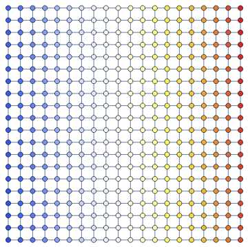
g=GridGraph[{100,100},VertexSizeLarge]

Out[]=

In[]:=

Attributes[SetTemperatures]={HoldFirst};SetTemperatures[g_,temperatures_]:=AnnotationValue[g,VertexWeight]=temperatures

In[]:=

GetTemperatures[g_]:=AnnotationValue[g,VertexWeight]

In[]:=

SetTemperatures[g,Range[1,20*20]]

Out[]=

{1,2,3,4,5,6,7,8,9,10,11,12,13,14,15,16,17,18,19,20,21,22,23,24,25,26,27,28,29,30,31,32,33,34,35,36,37,38,39,40,41,42,43,44,45,46,47,48,49,50,51,52,53,54,55,56,57,58,59,60,61,62,63,64,65,66,67,68,69,70,71,72,73,74,75,76,77,78,79,80,81,82,83,84,85,86,87,88,89,90,91,92,93,94,95,96,97,98,99,100,101,102,103,104,105,106,107,108,109,110,111,112,113,114,115,116,117,118,119,120,121,122,123,124,125,126,127,128,129,130,131,132,133,134,135,136,137,138,139,140,141,142,143,144,145,146,147,148,149,150,151,152,153,154,155,156,157,158,159,160,161,162,163,164,165,166,167,168,169,170,171,172,173,174,175,176,177,178,179,180,181,182,183,184,185,186,187,188,189,190,191,192,193,194,195,196,197,198,199,200,201,202,203,204,205,206,207,208,209,210,211,212,213,214,215,216,217,218,219,220,221,222,223,224,225,226,227,228,229,230,231,232,233,234,235,236,237,238,239,240,241,242,243,244,245,246,247,248,249,250,251,252,253,254,255,256,257,258,259,260,261,262,263,264,265,266,267,268,269,270,271,272,273,274,275,276,277,278,279,280,281,282,283,284,285,286,287,288,289,290,291,292,293,294,295,296,297,298,299,300,301,302,303,304,305,306,307,308,309,310,311,312,313,314,315,316,317,318,319,320,321,322,323,324,325,326,327,328,329,330,331,332,333,334,335,336,337,338,339,340,341,342,343,344,345,346,347,348,349,350,351,352,353,354,355,356,357,358,359,360,361,362,363,364,365,366,367,368,369,370,371,372,373,374,375,376,377,378,379,380,381,382,383,384,385,386,387,388,389,390,391,392,393,394,395,396,397,398,399,400}

In[]:=

GetTemperatures[g]

Out[]=

{1,2,3,4,5,6,7,8,9,10,11,12,13,14,15,16,17,18,19,20,21,22,23,24,25,26,27,28,29,30,31,32,33,34,35,36,37,38,39,40,41,42,43,44,45,46,47,48,49,50,51,52,53,54,55,56,57,58,59,60,61,62,63,64,65,66,67,68,69,70,71,72,73,74,75,76,77,78,79,80,81,82,83,84,85,86,87,88,89,90,91,92,93,94,95,96,97,98,99,100,101,102,103,104,105,106,107,108,109,110,111,112,113,114,115,116,117,118,119,120,121,122,123,124,125,126,127,128,129,130,131,132,133,134,135,136,137,138,139,140,141,142,143,144,145,146,147,148,149,150,151,152,153,154,155,156,157,158,159,160,161,162,163,164,165,166,167,168,169,170,171,172,173,174,175,176,177,178,179,180,181,182,183,184,185,186,187,188,189,190,191,192,193,194,195,196,197,198,199,200,201,202,203,204,205,206,207,208,209,210,211,212,213,214,215,216,217,218,219,220,221,222,223,224,225,226,227,228,229,230,231,232,233,234,235,236,237,238,239,240,241,242,243,244,245,246,247,248,249,250,251,252,253,254,255,256,257,258,259,260,261,262,263,264,265,266,267,268,269,270,271,272,273,274,275,276,277,278,279,280,281,282,283,284,285,286,287,288,289,290,291,292,293,294,295,296,297,298,299,300,301,302,303,304,305,306,307,308,309,310,311,312,313,314,315,316,317,318,319,320,321,322,323,324,325,326,327,328,329,330,331,332,333,334,335,336,337,338,339,340,341,342,343,344,345,346,347,348,349,350,351,352,353,354,355,356,357,358,359,360,361,362,363,364,365,366,367,368,369,370,371,372,373,374,375,376,377,378,379,380,381,382,383,384,385,386,387,388,389,390,391,392,393,394,395,396,397,398,399,400}

In[]:=

Attributes[NormalizeTemperatures]={HoldFirst};NormalizeTemperatures[g_]:=SetTemperatures[g,N[#/Max[#]]]&@GetTemperatures[g]

In[]:=

NormalizeTemperatures[g]

Out[]=

{0.0025,0.005,0.0075,0.01,0.0125,0.015,0.0175,0.02,0.0225,0.025,0.0275,0.03,0.0325,0.035,0.0375,0.04,0.0425,0.045,0.0475,0.05,0.0525,0.055,0.0575,0.06,0.0625,0.065,0.0675,0.07,0.0725,0.075,0.0775,0.08,0.0825,0.085,0.0875,0.09,0.0925,0.095,0.0975,0.1,0.1025,0.105,0.1075,0.11,0.1125,0.115,0.1175,0.12,0.1225,0.125,0.1275,0.13,0.1325,0.135,0.1375,0.14,0.1425,0.145,0.1475,0.15,0.1525,0.155,0.1575,0.16,0.1625,0.165,0.1675,0.17,0.1725,0.175,0.1775,0.18,0.1825,0.185,0.1875,0.19,0.1925,0.195,0.1975,0.2,0.2025,0.205,0.2075,0.21,0.2125,0.215,0.2175,0.22,0.2225,0.225,0.2275,0.23,0.2325,0.235,0.2375,0.24,0.2425,0.245,0.2475,0.25,0.2525,0.255,0.2575,0.26,0.2625,0.265,0.2675,0.27,0.2725,0.275,0.2775,0.28,0.2825,0.285,0.2875,0.29,0.2925,0.295,0.2975,0.3,0.3025,0.305,0.3075,0.31,0.3125,0.315,0.3175,0.32,0.3225,0.325,0.3275,0.33,0.3325,0.335,0.3375,0.34,0.3425,0.345,0.3475,0.35,0.3525,0.355,0.3575,0.36,0.3625,0.365,0.3675,0.37,0.3725,0.375,0.3775,0.38,0.3825,0.385,0.3875,0.39,0.3925,0.395,0.3975,0.4,0.4025,0.405,0.4075,0.41,0.4125,0.415,0.4175,0.42,0.4225,0.425,0.4275,0.43,0.4325,0.435,0.4375,0.44,0.4425,0.445,0.4475,0.45,0.4525,0.455,0.4575,0.46,0.4625,0.465,0.4675,0.47,0.4725,0.475,0.4775,0.48,0.4825,0.485,0.4875,0.49,0.4925,0.495,0.4975,0.5,0.5025,0.505,0.5075,0.51,0.5125,0.515,0.5175,0.52,0.5225,0.525,0.5275,0.53,0.5325,0.535,0.5375,0.54,0.5425,0.545,0.5475,0.55,0.5525,0.555,0.5575,0.56,0.5625,0.565,0.5675,0.57,0.5725,0.575,0.5775,0.58,0.5825,0.585,0.5875,0.59,0.5925,0.595,0.5975,0.6,0.6025,0.605,0.6075,0.61,0.6125,0.615,0.6175,0.62,0.6225,0.625,0.6275,0.63,0.6325,0.635,0.6375,0.64,0.6425,0.645,0.6475,0.65,0.6525,0.655,0.6575,0.66,0.6625,0.665,0.6675,0.67,0.6725,0.675,0.6775,0.68,0.6825,0.685,0.6875,0.69,0.6925,0.695,0.6975,0.7,0.7025,0.705,0.7075,0.71,0.7125,0.715,0.7175,0.72,0.7225,0.725,0.7275,0.73,0.7325,0.735,0.7375,0.74,0.7425,0.745,0.7475,0.75,0.7525,0.755,0.7575,0.76,0.7625,0.765,0.7675,0.77,0.7725,0.775,0.7775,0.78,0.7825,0.785,0.7875,0.79,0.7925,0.795,0.7975,0.8,0.8025,0.805,0.8075,0.81,0.8125,0.815,0.8175,0.82,0.8225,0.825,0.8275,0.83,0.8325,0.835,0.8375,0.84,0.8425,0.845,0.8475,0.85,0.8525,0.855,0.8575,0.86,0.8625,0.865,0.8675,0.87,0.8725,0.875,0.8775,0.88,0.8825,0.885,0.8875,0.89,0.8925,0.895,0.8975,0.9,0.9025,0.905,0.9075,0.91,0.9125,0.915,0.9175,0.92,0.9225,0.925,0.9275,0.93,0.9325,0.935,0.9375,0.94,0.9425,0.945,0.9475,0.95,0.9525,0.955,0.9575,0.96,0.9625,0.965,0.9675,0.97,0.9725,0.975,0.9775,0.98,0.9825,0.985,0.9875,0.99,0.9925,0.995,0.9975,1.}

In[]:=

ColorByInternalTemperature[g_]:=ColorByTemperature[g,GetTemperatures[g]]

In[]:=

ColorByInternalTemperature[g]

Out[]=

In[]:=

ColorByTemperature[g_,temperatures_]:=HighlightGraph[g,MapThread[Style,{VertexList[g],Map[ColorData["TemperatureMap"],temperatures]}]]

In[]:=

ListAnimate[{g,g,g,g,g}]

Out[]=

In[]:=

g

Out[]=

In[]:=

ListAnimate[Table[ColorByInternalTemperature[g],100]]

Out[]=

In[]:=

Table[g,2]

In[]:=

g

In[]:=

Table[RandomReal[],100]

Out[]=

{0.670039,0.485084,0.998206,0.667816,0.0218799,0.944035,0.881855,0.590729,0.871545,0.0885525,0.0866642,0.915112,0.43652,0.289185,0.630997,0.160342,0.760038,0.751826,0.525881,0.333667,0.044501,0.555605,0.755765,0.516203,0.476615,0.991612,0.739749,0.948589,0.373754,0.409902,0.96304,0.996546,0.20067,0.14545,0.519158,0.106787,0.136091,0.0181793,0.0435879,0.656578,0.88124,0.374613,0.398866,0.937661,0.755036,0.993684,0.996748,0.912976,0.575986,0.508083,0.01432,0.562618,0.21275,0.371477,0.6699,0.401753,0.0962863,0.850838,0.64523,0.488379,0.872293,0.899931,0.892373,0.468846,0.41338,0.063096,0.375492,0.981802,0.717503,0.567423,0.180118,0.45248,0.770596,0.769821,0.182089,0.227501,0.631988,0.780135,0.393047,0.128607,0.0506371,0.0036716,0.541328,0.435545,0.774793,0.456434,0.861841,0.976643,0.72642,0.613892,0.247511,0.709429,0.534959,0.725494,0.125309,0.133181,0.944277,0.206451,0.542094,0.760733}

In[]:=

ColorByRandomTemperature[g_]:=ColorByTemperature[g,Table[RandomReal[],VertexCount[g]]]

In[]:=

ListAnimate[Table[ColorByRandomTemperature[g],10]]

Out[]=

In[]:=

WM=ResourceFunction["WolframModel"]

Out[]=

[◼]	WolframModel

In[]:=

Universe7714=WM[{{{1,2,2},{3,1,4}}{{2,5,2},{2,3,5},{4,5,5}}},{{1,1,1},{1,1,1}},1000,"FinalState"];HG2G=ResourceFunction["HypergraphToGraph"]

Out[]=

[◼]	HypergraphToGraph

In[]:=

g7714=HG2G[Universe7714,VertexSizeLarge]

Out[]=

In[]:=

VertexCount[g7714]

Out[]=

1001

In[]:=

ColorByRandomTemperature[g7714]

Out[]=

In[]:=

ListAnimate[Table[ColorByRandomTemperature[g7714],50]]

Out[]=

Keywords

◼

Weyl

◼

Laplace-Beltrami

◼

Heat

◼

Riemannian

◼

Green

Acknowledgment

Mentor: Matthew Szudzik

Thanks to Matthew Szudzik, Jonathan Gorard and Daniel Sanchez for their assistance in developing this project.

References

◼

Arendt W, Nittka R, Peter W and Steiner F, Weyl’s Law: Spectral Properties of the Laplacian in Mathematics and Physics, Mathematical Analysis of Evolution, Information and Complexity (2009).

◼

Gorard, J,. Some Relativistic and Gravitational Properties of the Wolfram Model (2020).

◼

Ivrii, V., 100 Years of Weyl’s Law (2017).

◼

Reuter M., Wolter Franz-Enrich, Shenton M. and Niethammer Marc, Laplace-Beltrami Eigenvalues and Topological Features of Eigenfunctions for Statistical Shape Analysis (2009).

◼

Durhuus B., Hausdorff and Spectral DImensions of Infinite Random Graphs (2009).

◼

Stevenson, M. Weyl’s Law http://www-personal.umich.edu/~stevmatt/weyl_law.pdf (2014).

◼

Schmidt, F., The Laplace-Beltrami-Operator on Riemannian Manifolds.

◼

Wikipedia with respect to Weyl’s Law, Laplace-Beltrami Operator, Laplacian Matrix et al.

Weyl’s Law And The Wolfram Model Of Physics

Wolfram Community Post

Introduction

1. The Heat Equation

The Heat Equation PDE

Discretizing the Heat Equation

2. Weyl' s Law

Background

​Exploration of Weyl’s Law WIth Respect to Wolfram Model Graphs Using The Laplacian Operator

3. The Laplace-Beltrami Operator

Background

​The Laplace - Beltrami Operator For Graphs

4. Spectral Graph Theory

Spectral Graph Theory

5. Conclusions And Future Work

References

Complete project work

Heat Kernel

The Heat Equation

Temporal evolution using eigenfunction decomposition

Keywords

Acknowledgment

References

Exploration of Weyl’s Law WIth Respect to Wolfram Model Graphs Using The Laplacian Operator

The Laplace - Beltrami Operator For Graphs