Essays, Posts & Presentations

What constrains wildfire burn areas?

Assaad Mrad

Author

Assaad Mrad

Title

What constrains wildfire burn areas?

Description

A summer school project (2021) to identify the landscape features the limit wildfire spread

Category

Essays, Posts & Presentations

Keywords

California, Wildfires, Landscape, Open Street Maps

URL

http://www.notebookarchive.org/2021-07-61kkhb5/

DOI

https://notebookarchive.org/2021-07-61kkhb5

Date Added

2021-07-13

Date Last Modified

2021-07-13

File Size

18.7 megabytes

Supplements

2021-07-61kkhb5_Supplements.zip

Rights

Redistribution rights reserved

WOLFRAM SUMMER SCHOOL 2021

What constrains wildfire burn areas?

Introduction

The goal of this 3-week project is to identify features of the landscape that tend to constrain burn areas once a wildfire starts. As western North America once again suffers a record-breaking drought, an intense fire season is thought to ensue in the second half of 2021. The only semi-effective response to such fire forecasts is to manage vegetated lands with high amounts of fuel - plant biomass. Managing fuels means reducing the fuel loading to create fire breaks, stripes of barren land to limit the spread of the fire, or pruning lower tree branches to reduce the probability of fire crowning. We aim to improve these managements strategies by identifying landscape features, natural or artificial, that are effective in limiting fire spread in the goal of emulating them.

The hypothesis of this project is that wildfire burn areas are constrained by different landscape elements such as fuel availability, natural fuel breaks such as water bodies and topography and artificial fuel breaks such as roads and forest clearing. The objectives are to 1) visualize different landscape layers simultaneously with burn areas for a high-level exploration of our hypothesis, 2) define quantitative metrics to relate landscape layers to burn areas, 3) and develop statistical and mechanistic modeling tools to describe burn area shape and distribution.

While the analysis in this project applies to wildfires anywhere on Earth, we decided to limit the geographic range to California due to relatively better data accessibility and because of the severe fire season that will follow this year.

Outline

1

.

Data import, data wrangling, and function definitions

1

.

1

.

Burn perimeter data: data import and wrangling

1

.

2

.

Burn perimeter data: create California wildfires dataset

1

.

3

.

Vegetation Classification: data import and wrangling

1

.

4

.

Elevation: data import and wrangling

1

.

5

.

Function definitions for visualizing and describing the statistics of vegetation and elevation inside and around fires

1

.

6

.

Vector data: import roads and rivers overlying and surrounding wildfires

1

.

7

.

Function definitions for analyzing boundaries in vector form: roads and rivers

2

.

Vector boundaries

3

.

Raster data: vegetation classification

4

.

Machine Learning methods: vegetation classification

5

.

Machine Learning methods: vegetation and elevation combined

6

.

Future work: testing the wind-driven vs fuel-driven fire paradigms

7

.

Future work: weather data

An extensive resource for fire perimeters is the Monitoring Trends in Burn Severity (MTBS) website. On the website, one can download the raw data from the Burned Areas Boundaries Dataset . I downloaded the zip file and put it in the same folder as this notebook. This dataset contains the perimeters of all reported burns, including wildfires and prescribed fires, in the United States from 1984 to 2019. This data will be imported and wrangled in the “Import burn perimeter data: data wrangling” section. The perimeter data will then be subset to only include California wildfires and will be analyzed in “Import burn perimeter data: data analysis” section.

Data import, data wrangling, and function definitions

Burn perimeter data: data import and wrangling


Burn perimeter data: create California wildfires dataset


Vegetation Classification: data import and wrangling


Elevation: data import and wrangling


Function definitions for visualizing and describing the statistics of vegetation and elevation inside and around fires


Vector data: import roads and rivers overlying and surrounding wildfires

Load from .wxf file

In[]:=

{roadMapsByType,roadPolyRas,boundaryByType,morphCompNum}=Import[NotebookDirectory[]<>"communityPostVector.wxf"];

Define thickness of each vector element in the “getRoadMap” function below

In[]:=

thicknesses=<|"road_primary"->0.005,"road_primary_ramp"->0.005,"road_primary_bridge"->0.005,"road_motorway"->0.005,"road_motorway_ramp"->0.005,"road_motorway_bridge"->0.005,"road_secondary"->0.003,"road_secondary_ramp"->0.003,"road_secondary_bridge"->0.003,"road_tertiary"->0.002,"road_tertiary_ramp"->0.002,"road_tertiary_bridge"->0.002,"road_minor"->0.001,"road_trunk"->0.001,"waterway_river"->0.005,"waterway_canal"->0.005|>;

Function to return a rasterized map of roads and rivers overlying and surrounding fires

In[]:=

getRoadMap[proj_,bounds_,dims_,opts___]:=With[{map=GeoGraphics[opts,PlotRange->bounds,GeoProjectionproj,GeoBackground->"VectorMinimal",GeoZoomLevel12,BackgroundBlack]},Rasterize[map/.{Annotation[{style_,prim_},layer:{"line",lt_,_},type_]:>If[!KeyExistsQ[thicknesses,lt],Nothing,Annotation[{Directive[Antialiasing->False,White,Thickness[thicknesses[lt]]],prim},layer,type]],Annotation[{style_,prim_},layer_,type_]:>Nothing},RasterSize->dims,BackgroundBlack]]

Example for the RUSH fire of 2012:

In[]:=

getRoadMap["Mercator",GIS`RangeTransformation[getBoundingBox[dsCaPoly[2,"Geometry"]],proj->"Mercator"],{1000,1000}]

Out[]=

Function to return a rasterized map of either roads or rivers

This function will be used to determine the most effective types of boundaries to wildfires

In[]:=

getRoadMapByType[proj_,bounds_,dims_,types_,opts___]:=With[{map=GeoGraphics[opts,PlotRange->bounds,GeoProjectionproj,GeoBackground->"VectorMinimal",GeoZoomLevel12,BackgroundBlack]},Rasterize[map/.{Annotation[{style_,prim_},layer:{"line",lt_,_},type_]:>If[!StringMatchQ[lt,types],Nothing,Annotation[{Directive[Antialiasing->False,White,Thickness[0.001]],prim},layer,type]],Annotation[{style_,prim_},layer_,type_]:>Nothing},RasterSize->dims,BackgroundBlack]]

getType is different from getRoadMapByType in that it is fed a map instead of computing it itself

In[]:=

getType[map_,dims_,types_]:=Rasterize[map/.{Annotation[{style_,prim_},layer:{"line",lt_,_},type_]:>If[!StringMatchQ[lt,types],Nothing,Annotation[{Directive[Antialiasing->False,White,Thickness[0.001]],prim},layer,type]],Annotation[{style_,prim_},layer_,type_]:>Nothing},RasterSize->dims,BackgroundBlack]

Example for the Happy Camp Complex of 2014 for roads:

In[]:=

getRoadMapByType["Mercator",GIS`RangeTransformation[getBoundingBox[dsCaPoly[16,"Geometry"]],proj->"Mercator"],{300,300},___~~"road"~~__]

Out[]=

Function to rasterize a polygon of a burn area to Highlight relevant vectors in (colored) road maps

In[]:=

roadRasterize[geom_]:=ColorConvert[Rasterize[Graphics[Style[Normal@geom,AntialiasingFalse],PlotRangegetBoundingBox[geom]],RasterSize{1000,1000}],"Grayscale"]

Compute roadMaps, roadMapsColored, and rasterized fire polygons for all California wildfires since 2001

In[]:=

(*roadPolyRas=ResourceFunction["DynamicMap"][roadRasterize[dsCaPoly[#,"Geometry"]]&,Range[Length[dsCaPoly]]];*)

In[]:=

(*roadMapsByType2=Table[With[{map=GeoGraphics[PlotRange->GIS`RangeTransformation[getBoundingBox[dsCaPoly[i,"Geometry"]],proj->"Mercator"],GeoProjection"Mercator",GeoBackground->"VectorMinimal",GeoZoomLevel12,BackgroundBlack]},{getType[map,{300,300},___~~"road"~~__],getType[map,{300,300},___~~"waterway"~~__]}],{i,Range[201,400]}];*)

Save road

In[]:=

(*BinaryWrite[NotebookDirectory[]<>"roadMapsByType2.wxf",ExportByteArray[roadMapsByType2,"WXF"]];*)

In[]:=

(*Close[NotebookDirectory[]<>"roadMapsByType2.wxf"];*)

In[]:=

(*roadMaps=ResourceFunction["DynamicMap"][With[{bbEqui=GIS`RangeTransformation[getBoundingBox[dsCaPoly[#,"Geometry"]],proj->"Mercator"]},ColorConvert[getRoadMap["Mercator",bbEqui,{1000,1000}],"Grayscale"]]&,Range[Length[dsCa]]];*)

In[]:=

(*roadMapsColored=ResourceFunction["DynamicMap"][With[{bbEqui=GIS`RangeTransformation[getBoundingBox[dsCaPoly[#,"Geometry"]],proj->"Mercator"]},getRoadMapColored["Mercator",bbEqui,{300,300}]]&,Range[Length[dsCa]]];*)

Function definitions for analyzing boundaries in vector form: roads and rivers

Function to get fraction of boundaries bounded by each vector component using the roadMapsByType

In[]:=

boundaryTypes[fireRas_,map_]:=Module{imDia=Dilation[map,DiskMatrix[0.5]],fireRasResized=EdgeDetect[ImageResize[fireRas,{300,300}],1],boundaryLength,boundTypeCounts},boundaryLength=ImageMeasurements[fireRasResized,"Total"];boundTypeCounts=ImageMeasurements[Binarize[fireRasResized-ColorSeparate[imDia,"R"],0.5],"Total"];1-

boundTypeCounts

boundaryLength



Compute the boundary types for the largest 400 fires in California since 2000

In[]:=

(*boundaryByType=ResourceFunction["DynamicMap"][{boundaryTypes[roadPolyRas[[#]],roadMapsByType[[#,1]]],boundaryTypes[roadPolyRas[[#]],roadMapsByType[[#,2]]]}&,Range[400]];*)

Function to calculate the number of morphological components formed by roads or rivers

In[]:=

getMorphCompNum[fireRas_,map_]:=Module[{morphComp=MorphologicalComponents[ImageSubtract[ColorNegate@ImageResize[fireRas,{300,300}],Dilation[map,DiskMatrix[2]]],0.9],selectComps},selectComps=Select[Tally[Flatten[morphComp]],#[[2]]>100&][[All,1]];Length[selectComps]-1]

Compute the number of morphological components for the largest 400 fires in California since 2000

In[]:=

(*morphCompNum=ResourceFunction["DynamicMap"][{getMorphCompNum[roadPolyRas[[#]],roadMapsByType[[#,1]]],getMorphCompNum[roadPolyRas[[#]],roadMapsByType[[#,2]]]}&,Range[400]];*)

Function to plot morphological components containing more than 100 pixels

In[]:=

plotMorphComp[fireRas_,map_]:=Module[{morphCompRanch=MorphologicalComponents[ImageSubtract[ColorNegate@ImageResize[fireRas,{300,300}],Dilation[map,DiskMatrix[2]]],0.9],selectComps},selectComps=Select[Tally[Flatten[morphCompRanch]],#[[2]]>100&][[All,1]];Colorize[morphCompRanch/.(x_Integer/;(!MemberQ[selectComps,x])->0),ImageSizeSmall]]

Example for the Ranch fire of 2012 for roads:

In[]:=

plotMorphComp[roadPolyRas[[1]],roadMapsByType[[1,1]]]

Out[]=

Save files necessary for vector analysis in community post


Vector boundaries

In[]:=

GeoGraphics{EdgeForm[Black],FaceForm[Red],Tooltip[#3,#1<>", "<>DateString@#2]&@@@Query[;;60,{"IncidName","IgDate","Geometry"}][dsCa]},GeoRange->

California, United States

ADMINISTRATIVE DIVISION



Out[]=

Variable effectiveness of roads and rivers as barriers

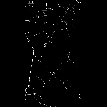
The effectiveness of roads and rivers as barriers to wildfire spread varies from fire to fire. From some of the most intense fires in the presence of wind, the creation and transport of embers by wind can spread a fire across wide fire breaks like roads and rivers. In that case, what one sees is similar to the left panel of the figure below where the Ranch fire spreads across multiple roads, colored in magenta. An equivalent view of the same phenomenon is that these roads divide the fire raster, colored in black, into multiple disconnected components which we will expand upon below. Rivers are not primary features of that landscape as they are sparse and only border 6.1% of the fire in the case of the Ranch fire. From the vector map on the right panel, one can see that water bodies occasionally block fires.

The Ranch fire of 2018: the presence of roads does not guarantee containment

In[]:=

Grid[{{"",Style["Roads",18],Style["Rivers",18],Style["Map",18]},{Rotate[Style["Boundary %",18],π/2],Style[NumberForm[boundaryByType[[1,1]]*100,2],16],Style[NumberForm[boundaryByType[[1,2]]*100,2],16],""},{Rotate[Style["Maps and rasters",18],π/2],HighlightImage[ImageResize[roadPolyRas[[1]],{300,300}],Thinning[roadMapsByType[[1,1]]],ImageSize->Small,ImagePadding10],HighlightImage[ImageResize[roadPolyRas[[1]],{300,300}],{Blue,Thinning[roadMapsByType[[1,2]]]},ImageSize->Small,ImagePadding10],GeoGraphics[dsCa[1,"Geometry"],GeoBackground"VectorMinimal",GeoZoomLevel12,ImageSizeSmall]}}]

Out[]=

	Roads	Rivers	Map
Boundary %	41.	6.1
Maps and rasters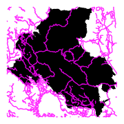

Roads are a more effective barrier in the case of the Happy Camp Complex according to the left panel in the figure below. This is due to roads only dividing the complex into 3 regions, indicating that the fire jumped across 2 roads at most only even though roads bordered 47% of the fire, more than the Ranch fire above. An important landscape feature around many fires is that roads and rivers are often co-located as seen by comparing the panels below. This might confound the analysis of the effectiveness of roads versus rivers as fire barriers.

The Happy Camp Complex of 2014: a case where roads and rivers are effective wildfire barriers

In[]:=

Grid[{(*{Style["The Happy Camp Complex of 2014: a case where roads and rivers are effective wildfire barriers",18],SpanFromLeft,SpanFromLeft},*){"",Style["Roads",18],Style["Rivers",18],Style["Map",18]},{Rotate[Style["Boundary %",18],π/2],Style[NumberForm[boundaryByType[[16,1]]*100,2],16],Style[NumberForm[boundaryByType[[16,2]]*100,2],16],""},{Rotate[Style["Maps and rasters",18],π/2],HighlightImage[ImageResize[roadPolyRas[[16]],{300,300}],Thinning[roadMapsByType[[16,1]]],ImageSize->Small,ImagePadding10],HighlightImage[ImageResize[roadPolyRas[[16]],{300,300}],{Blue,Thinning[roadMapsByType[[16,2]]]},ImageSize->Small,ImagePadding10],GeoGraphics[dsCa[16,"Geometry"],GeoBackground"VectorMinimal",GeoZoomLevel12,ImageSizeSmall]}}]

Out[]=

	Roads	Rivers	Map
Boundary %	47.	31.
Maps and rasters

We can use the idea of splitting fire rasters into morphological components based on road and river vectors to quantify their effectiveness. When fires jump more often across roads, they are split into more morphological components. Thus, a smaller number of components indicates a more effective barrier given a certain boundary percentage. The figure below shows the same two example fires above but split into morphological components based on road vectors. The Ranch fire has 14 morphological components compared to the Happy Camp Complex’s 3. This result quantifies the observation we made above that roads are a more effective barrier to fire spread in case of the latter. This statement is based also on the proportion of the fire boundaries being occupied by roads being similar, 41 and 47%.

Roads splitting fire rasters into multiple morphological components: a measure of effectiveness

In[]:=

Grid[{{"",Style["Ranch fire",18],Style["Happy Camp Complex",18]},{Rotate[Style["#",18],π/2],Style[morphCompNum[[1,1]],16],Style[morphCompNum[[16,1]],16]},{Rotate[Style["Morphological components",18],π/2],plotMorphComp[roadPolyRas[[1]],roadMapsByType[[1,1]]],plotMorphComp[roadPolyRas[[16]],roadMapsByType[[16,1]]]}}]

Out[]=

	Ranch fire	Happy Camp Complex
#	14	3
Morphological components

In[]:=

Rasterize[Grid[{{plotMorphComp[roadPolyRas[[1]],roadMapsByType[[1,1]]],plotMorphComp[roadPolyRas[[16]],roadMapsByType[[16,1]]]}}]]

Out[]=

Statistics over the largest 400 fires in California since year 2000


Raster data

Explore dominant vegetation types inside and around fires

Compute dominant vegetation type inside and around the fire


Import if already saved

In[]:=

dominantVegClassAssociation=Association[Import[NotebookDirectory[]<>"burnVegClassAssociationType2.wxf"]/.{x_,y_}:>Association[x,y]];

Example for Ranch fire of 2012

In[]:=

dominantVegClassAssociation[[;;2]]

Out[]=

{39.269,-122.775,427048}inside{Evergreen Needleleaf Forests,0.387276},around{Woody Savannas,0.28502},{40.603,-120.09,306811}inside{Grasslands,0.999701},around{Grasslands,0.991457}

The Keys for this association are {lat, lon, acres}. These were was used in an earlier version of the notebook to create a classifier for predicting vegetation dominance based on them. But then I opted against them because the good results were probably artefacts of dominant vegetation being a function of topography, location, and elevation inherently.

Save burnVegClassAssociation as WXF file


Filter out cases where dominant vegetation is “unclassified”

In[]:=

dominantVegClassAssociationFiltered=Query[Select[StringQ[#inside[[1]]]&&StringQ[#around[[1]]]&&!StringMatchQ[#around[[1]],"Unclassified"]&]]@Association[dominantVegClassAssociation/.{x_,y_}:>Association[x,y]];

Vegetation bar plot inside and around burn areas

In[]:=

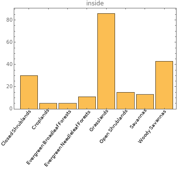
Grid[{{Style["Dominant vegetation types by number of wildfires",18],SpanFromLeft},Function[i,BarChart[KeySort@Counts@DeleteMissing@Query[Values,#[i][[1]]&][dominantVegClassAssociationFiltered],ChartLabelsPlaced[Automatic,{{0.5,0},{0.9,1}},Rotate[#,(2/7)Pi]&],FrameTrue,PlotLabeli,ImageSizeMedium]]/@{"inside","around"}}]

Out[]=

Dominant vegetation types by number of wildfires

Dense Herbaceous vegetation class dominates both inside and around the forest, this is not surprising as this is the most abundant vegetation class in California. The second most abundant class is Evergreen Needleleaf Forests.

Vegetation bar plot inside and around burn areas when they are different

In[]:=

burnVegDiff=Query[Select[!StringMatchQ[#inside[[1]],#around[[1]]]&]][dominantVegClassAssociationFiltered];

In[]:=

Grid[{{Style["Dominant vegetation types when they are different inside and around each fire",18],SpanFromLeft},Function[i,BarChart[KeySort@Counts@DeleteMissing@Query[Values,#[i][[1]]&][burnVegDiff],ChartLabelsPlaced[Automatic,{{0.5,0},{0.9,1}},Rotate[#,(2/7)Pi]&],FrameTrue,PlotLabeli,ImageSizeMedium]]/@{"inside","around"}}]

Out[]=

Dominant vegetation types when they are different inside and around each fire

Even when the dominant vegetation types inside and around fires are different, the Grasslands type still is the most abundant in terms of the number of fires (inside area) it dominates. However, the dominant types around fires are Evergreen Broadleaf Forests, Savannas, and grasslands.

Create an array of vegetation probability within and around each fire

The idea here is to create an array of vegetation classes for each fire such that each element of the array is a percentage of all pixels inside the burn area. A background association “vegClassBackground” is created to get the same array size for each fire such that we will get a matrix in the end.

In[]:=

vegClassBackground=KeySort[Association[(#->0)&/@Values@vegClass]]

Out[]=

Closed Shrublands0,Cropland/Natural Vegetation Mosaics0,Croplands0,Deciduous Broadleaf Forests0,Evergreen Broadleaf Forests0,Evergreen Needleleaf Forests0,Grasslands0,Mixed Forests0,Non-Vegetated Lands0,Open Shrublands0,Permanent Wetlands0,Savannas0,Unclassified0,Urban and Built-up Lands0,Water Bodies0,Woody Savannas0

In[]:=

(*vegMatrixInside=With[{temp=KeySort[Merge[{getVegList[vegClass,burnAreaVegClass[Lookup[#,"Geometry"],targetRange,lcImageProj[Lookup[#,"IgDate"]["Year"]],10],"inside"],vegClassBackground},Total]]},Values[N[temp/Total[temp]]]]&/@Normal@dsCaPoly;*)

In[]:=

(*vegMatrixAround=With[{temp=KeySort[Merge[{getVegList[vegClass,burnAreaVegClass[Lookup[#,"Geometry"],targetRange,lcImageProj[Lookup[#,"IgDate"]["Year"]],10],"around"],vegClassBackground},Total]]},Values[N[temp/Total[temp]]]]&/@Normal@dsCaPoly;*)

In[]:=

{vegMatrixInside,vegMatrixAround}=Import[NotebookDirectory[]<>"vegMatricesType2.wxf"];

In case matrices were just computed, save as WXF file


Machine Learning methods: vegetation classification

The goal is to create a classifier to predict whether a given vegetation list is inside or around a fire. For the first try, only have vegetation data plugged in in the form of a matrix according to vegMatrixInside and vegMatrixOutside

Remove any arrays that have any “unclassified” pixels and drop any element because array elements sum to 1 without loss of information

In[]:=

unclassifiedPos=First@First@Position[Keys[vegClassBackground],"Unclassified"]

Out[]=

13

In[]:=

vegMatrixInsideReduced=Drop[Select[vegMatrixInside,#[[unclassifiedPos]]==0&],None,{1}];

In[]:=

vegMatrixAroundReduced=Drop[Select[vegMatrixAround,#[[unclassifiedPos]]==0&],None,{1}];

Join matrices by threading a Rule between each array and “inside” or “around”

In[]:=

vegMatrixAll=Join[Thread[vegMatrixInsideReduced->"inside"],Thread[vegMatrixAroundReduced->"around"]];

Do a 70-30 split for training and validation

In[]:=

testVegMat=RandomSample[vegMatrixAll,Round[Length[vegMatrixAll]*0.3]];trainingVegMat=Complement[vegMatrixAll,testVegMat];

Train a classifier

In[]:=

insideOrAround=Classify[trainingVegMat,PerformanceGoal"Quality",ValidationSettestVegMat]

Out[]=

ClassifierFunction

Input type: NumericalVector

(length: 15)

Classes: around,inside



Evaluate performance

In[]:=

Information[insideOrAround]

Out[]=

Classifier information

Data type	NumericalVector (length: 15)
Classes	around , inside
Accuracy	(61.8 ± 2.2 ) %
Method	RandomForest
Single evaluation time	8.99 ms/example
Batch evaluation speed	8.4 examples/ms
Loss	0.677 ± 0.0046
Model memory	614. kB
Training examples used	1107 examples
Training time	3.94 s

From the information above, the accuracy of the classifier was ~63% which is a bit higher than the baseline accuracy of 50%. The baseline accuracy is 50% because the dataset is balanced which means that there are as many arrays for inside and for around the fire.

In[]:=

ClassifierMeasurements[insideOrAround,testVegMat,"AreaUnderROCCurve"]

Out[]=

around0.691774,inside0.693697

The Area under the ROC is about 70% which is not bad but not too good.

In[]:=

ClassifierMeasurements[insideOrAround,testVegMat,"ConfusionMatrixPlot"]

Out[]=

A large number is misclassified.

Future work: Do a scalewise variation. Pick incrementally larger study areas. (Tirtha) Split vegetation into coastal and inland to evaluate fuel-driven vs wind-driven fires. Drop fires that have water bodies and barren lands around them to see if classifier still gets 63% accuracy. We suspect the relatively high accuracy might be an artefact of that.

Trying an an unsupervised method, DimensionReduce, to see if there is a clear split

In[]:=

features=DimensionReduce[Join[vegMatrixInsideReduced,vegMatrixAroundReduced],Method->"TSNE"];

In[]:=

ListPlot[With[{len=features//Length},{features[[;;Round[len/2]]],features[[Round[len/2]+1;;]]}]]

Out[]=

There is no clear split but Stephen thinks there might be something behind this structure and that it is worth studying more deeply.

Machine Learning methods: vegetation and elevation combined

Visualization and computation

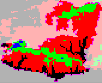
Visualize elevation raster for the WOOLSEY fire of 2018

In[]:=

viz[burnAreaRasIm[dsCaPoly[21,"Geometry"],targetRange,elevImProj]]

Out[]=

highlightWhere

inside

around

outside

Compute mean and std of elevation and slope of each fire


In case meanElevList was just computed, save as WXF file


Elevation statistics for California wildfires

In[]:=

Histogram[meanStdElevAroundList[[All,1]],FrameTrue,FrameLabel{{"Mean fire elevation",None},{"Fire frequency","Histogram of mean fire elevations"}}]

Out[]=

Classifier to predict whether a given vegetation list is inside or around a fire including mean fire elevation data as well as vegetation

Define whitening transformation

This is to drop the infinite precision assumption and make computations faster.

In[]:=

whiteningTransformation[list_]:=With{listFast=list*1.0},Transpose@

Transpose@listFast-Mean[listFast]

StandardDeviation[listFast]

;

Remove any arrays that have any “unclassified” pixels and drop any element because array elements sum to 1 without loss of information

In[]:=

vegElevMatrixInside=Drop[Select[Join[vegMatrixInside,Partition[whiteningTransformation[meanStdElevList[[All,1]]],1],2],#[[unclassifiedPos]]==0&],None,{1}];

In[]:=

vegElevMatrixAround=Drop[Select[Join[vegMatrixAround,Partition[whiteningTransformation[meanStdElevAroundList[[All,1]]],1],2],#[[unclassifiedPos]]==0&],None,{1}];

Combine matrices and thread rules

In[]:=

vegElevMatrixAll=Join[Thread[vegElevMatrixInside->"inside"],Thread[vegElevMatrixAround->"around"]];

Split into training and validation 70-30

In[]:=

testVegElevMat=RandomSample[vegElevMatrixAll,Round[Length[vegElevMatrixAll]*0.3]];trainingVegElevMat=Complement[vegElevMatrixAll,testVegElevMat];

Train classifier

In[]:=

insideOrAroundElev=Classify[trainingVegElevMat,PerformanceGoal"Quality",ValidationSettestVegElevMat]

Out[]=

ClassifierFunction

Input type: NumericalVector

(length: 16)

Classes: around,inside



In[]:=

Information[insideOrAroundElev]

Out[]=

Classifier information

Data type	NumericalVector (length: 16)
Classes	around , inside
Accuracy	(65.5 ± 3.0 ) %
Method	GradientBoostedTrees
Single evaluation time	7.11 ms/example
Batch evaluation speed	10.9 examples/ms
Loss	0.650 ± 0.031
Model memory	404. kB
Training examples used	1181 examples
Training time	3.46 s

Accuracy has improved by 4%

In[]:=

ClassifierMeasurements[insideOrAroundElev,testVegElevMat,"AreaUnderROCCurve"]

Out[]=

around0.738152,inside0.738333

AUC has increased by 5%

In[]:=

ClassifierMeasurements[insideOrAroundElev,testVegElevMat,"ConfusionMatrixPlot"]

Out[]=

Classifier that includes mean fire slope

Compute matrices with the same dropping of “unclassified” cases

In[]:=

vegSlopeMatrixInside=Drop[Select[Join[vegMatrixInside,Partition[whiteningTransformation[meanStdSlopeList[[All,1]]],1],2],#[[unclassifiedPos]]==0&],None,{1}];

In[]:=

vegSlopeMatrixAround=Drop[Select[Join[vegMatrixAround,Partition[whiteningTransformation[meanStdSlopeList[[All,1]]],1],2],#[[unclassifiedPos]]==0&],None,{1}];

Combine matrices

In[]:=

vegSlopeMatrixAll=Join[Thread[vegSlopeMatrixInside->"inside"],Thread[vegSlopeMatrixAround->"around"]];

Training and testing data

In[]:=

testVegSlopeMat=RandomSample[vegSlopeMatrixAll,Round[Length[vegSlopeMatrixAll]*0.3]];trainingVegSlopeMat=Complement[vegSlopeMatrixAll,testVegSlopeMat];

Train classifier

In[]:=

insideOrAroundSlope=Classify[trainingVegSlopeMat,PerformanceGoal"Quality",Method"GradientBoostedTrees"]

Out[]=

ClassifierFunction

Input type: NumericalVector

(length: 16)

Classes: around,inside



Classifier information

In[]:=

Information[insideOrAroundSlope]

Out[]=

Classifier information

Data type	NumericalVector (length: 16)
Classes	around , inside
Accuracy	(64. ± 4. ) %
Method	GradientBoostedTrees
Single evaluation time	11. ms/example
Batch evaluation speed	13.6 examples/ms
Loss	0.668 ± 0.031
Model memory	438. kB
Training examples used	1196 examples
Training time	3.81 s

In[]:=

ClassifierMeasurements[insideOrAroundSlope,testVegSlopeMat,"AreaUnderROCCurve"]

Out[]=

around0.730713,inside0.730773

Classifier with mean elevation seems to fare better when it comes to AUC.

In[]:=

ClassifierMeasurements[insideOrAroundSlope,testVegSlopeMat,"ConfusionMatrixPlot"]

Out[]=

Future work: Include only slopes around the fire and differentiate whether they are going into or out of the fires.

Future work: testing the wind-driven vs fuel-driven fire paradigms

Recently, California fires were categorized as either wind-driven or fuel driven (Keeley & Syphard, 2019). Typically in the mid- and north-western parts of the state, fuel-driven fires occur in regions where fire suppression and silvicultural practices have led to the accumulation of fuels where, historically, many fires occurred. Fuel-driven fires are usually caused by lightning and occur in the summer months (July & August). In contrast, wind-driven fires occur on the eastern part of the state. In the autumn, a high pressure system in the interior basin and a low pressure system over the Pacific means that high-speed offshore winds develop. These winds tend to intensify small fires, typically caused by humans, to form large conflagrations.

Examples of fuel driven fires are the Rush (2012), Rim (2013), Rough (2015), and Marble Cone (2007) fires

Examples of wind-driven fires are the Thomas (2017), Witch (2007), Camp (2018) fires

Future work: weather data

Use WeatherData. DayMet by ORNL. Daily meteorological values at surface based on observations. Temp (min and max; better for heat stress; deviation from climatic average; pentads: multiples of 5 days), Rainfall (last time, and cumulative).

Lauren: LandSurface index gives an idea of vegetation stress

->

probability for my vegetation to burn. What type of soil do you have? If you have a lot of organic matter, then it plays a big role. SOM (Soil Organic Matter). if SOM % datasets don’t exist a lot, knowing soil porosity would be a good substitute.

Morphological components and see how many regions are covered to see how many roads the fire

Weather radar and precipitation.

In[]:=

dsCa[1,{"BurnBndLat","BurnBndLon","IgDate"}]

Out[]=

BurnBndLat	39.269
BurnBndLon	-122.775
IgDate	Fri 27 Jul 2018

In[]:=

Normal@Values@dsCa[1,{"BurnBndLat","BurnBndLon"}]

Out[]=

{39.269,-122.775}

In[]:=

dsCa[5,"IgDate"]+

Out[]=

Mon 19 Aug 2013

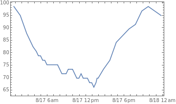
AirTemperatureDataToExpression@Normal@Values@dsCa[5,{"BurnBndLat","BurnBndLon"}],dsCa[5,"IgDate"],dsCa[5,"IgDate"]+

1

days



Out[]=

TimeSeries

Time: 17 Aug 2013 00:45:00 to 17 Aug 2013 23:45:00
Data points: 44



DateListPlot[%]

Out[]=

In[]:=

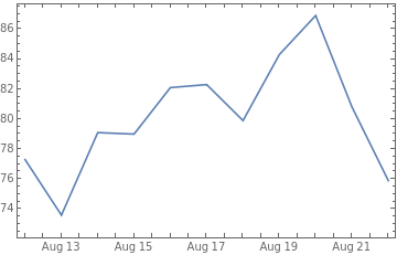
AirTemperatureDataToExpression@Normal@Values@dsCa[5,{"BurnBndLat","BurnBndLon"}],dsCa[5,"IgDate"]-

5

days

,dsCa[5,"IgDate"]+

5

days

,"Day"

Out[]=

TimeSeries

Time: 12 Aug 2013 to 22 Aug 2013
Data points: 11



In[]:=

DateListPlot[%]

Out[]=

In[]:=

WindSpeedDataToExpression@Normal@Values@dsCa[5,{"BurnBndLat","BurnBndLon"}],dsCa[5,"IgDate"]-

5

days

,dsCa[5,"IgDate"]+

5

days

,"Day"

Out[]=

TimeSeries

Time: 12 Aug 2013 to 22 Aug 2013
Data points: 11



In[]:=

DateListPlot[%]

Out[]=

WindSpeedDataToExpression@Normal@Values@dsCa[5,{"BurnBndLat","BurnBndLon"}],dsCa[5,"IgDate"]-

5

days

,dsCa[5,"IgDate"]+

5

days

,"Day"

In[]:=

WeatherData[ToExpression@Normal@Values@dsCa[2,{"BurnBndLat","BurnBndLon"}],"Temperature",dsCa[2,"IgDate"],TimeZone->"America/Los_Angeles"]

Out[]=

TimeSeries

Time: 12 Aug 2012 00:55:00 to 12 Aug 2012 23:55:00
Data points: 25



In[]:=

DateListPlot[%]

Out[]=

In[]:=

$TimeZone

Out[]=

-4.

In[]:=

WeatherData["Chicago","Temperature",Yesterday]

Out[]=

TimeSeries

Time: 10 Jul 2021 00:53:00 to 10 Jul 2021 23:53:00
Data points: 29



In[]:=

DateListPlot[%]

Out[]=

Cite this as: Assaad Mrad, "What constrains wildfire burn areas?" from the Notebook Archive (2021), https://notebookarchive.org/2021-07-61kkhb5