Essays, Posts & Presentations

Hidden Figures: Modern Approaches to Orbit and Reentry Calculations

Jeffrey Bryant

Author

Jeffrey Bryant

Title

Hidden Figures: Modern Approaches to Orbit and Reentry Calculations

Description

Hidden Figures: Modern Approaches to Orbit and Reentry Calculations

Jeff Bryant, Research Programmer, Wolfram|Alpha Scientific Content

Paco Jain, Research Programmer, Wolfram|Alpha Scientific Content

Michael Trott, Chief Scientist

The movie Hidden Figures was released in theaters recently and has been getting good reviews. It also deals with an important time in US history, touching on a number of topics, including civil rights and the Space Race. The movie details the hidden story of Katherine Johnson and her coworkers (Dorothy Vaughan and Mary Jackson) at NASA during the Mercury missions and the United States’ early explorations into manned space flight. The movie focuses heavily on the dramatic civil rights struggle of African American women in NASA at the time, and these struggles are set against the number-crunching ability of Johnson and her coworkers. Computers were in their early days at this time, so Johnson and her team’s ability to perform complicated navigational orbital mechanics problems without the use of a computer provided an important sanity check against the early computer results.

RowShow

Hidden Figures

MOVIE



image

,ImageSize101," ",Show

Katherine Johnson-like curve

POPULAR CURVE



image

,AxesFalse,BackgroundLightBlue,ImageSize120

I will touch on two aspects of her scientific work that were mentioned in the film: orbit calculations and reentry calculations. For the orbit calculation, I will first exactly follow what Johnson did and then compare with a more modern, direct approach utilizing an array of tools made available with the Wolfram Language. Where the movie mentions the solving of differential equations using Euler’s method, I will compare this method with more modern ones in an important problem of rocketry: computing a reentry trajectory from the rocket equation and drag terms (derived using atmospheric model data obtained directly from within the Wolfram Language).

The movie doesn't focus much on the math details of the types of problems Johnson and her team dealt with, but for the purposes of this blog, I hope to provide at least a flavor of the approaches one might have used in Johnson’s day compared to the present.

◼

Placing a Satellite over a Selected Position

One of the earliest papers that Johnson coauthored, “Determination of Azimuth Angle at Burnout for Placing a Satellite over a Selected Earth Position,” deals with the problem of making sure that a satellite can be placed over a specific Earth location after a specified number of orbits, given a certain starting position (e.g. Cape Canaveral, Florida) and orbital trajectory. The approach that Johnson’s team used was to determine the azimuthal angle (the angle formed by the spacecraft’s velocity vector at the time of engine shutoff with a fixed reference direction, say north) to fire the rocket in, based on other orbital parameters. This is an important step in making sure that an astronaut is in the correct location for reentry to Earth.

Constants and Initial Processing

In the paper, Johnson defines a number of constants and input parameters needed to solve the problem at hand. One detail to explain is the term “burnout,” which refers to the shutoff of the rocket engine. After burnout, orbital parameters are essentially “frozen,” and the spacecraft moves solely under the Earth’s gravity (as determined, of course, through Newton’s laws). In this section, I follow the paper’s unit conventions as closely as possible.

v1=25761.34560;(*satellitevelocityinft/min*)r1=21637933.;(*circularorbitradiusinfeet*)γ1=0.5;(*elevationanglebetweenlocalhorizonandvelocityvectorindegrees*)vc=25506.2860;(*circularorbitvelocityinft/min*)poverr1=1.020022269;(*pisthesemilatusrectumoftheorbitellipse*)a=22081775.57;(*semimajoraxisoforbitinfeet*)tθ1=5.842;(*t[θ1]isthetimefromperigeeforθ1inmin,whereθ1isangleinorbitplanebetweenperigeeandburnout*)g0=115991.595;(*accelerationduetogravityft/min^2*)R=2.09022610^7;(*Earthradiusinfeet*)(*launchcoordinates*)ϕ1=28.50;(*launchlatitude*)λ1=279.45;(*launchlongitude*)ϕ2=34.00;(*intendedpassoverlatitude*)λ2=241.00;(*intendedpassoverlongitude*)n=3;(*numberoforbits*)ωCapitale=0.25068(*angularvelocityofEarthindegrees/min*);

For convenience, some functions are defined to deal with angles in degrees instead of radians. This allows for smoothly handling time in angle calculations:

SinDegree[x_]:=Sin[xDegree]CosDegree[x_]:=Cos[xDegree]TanDegree[x_]:=Tan[xDegree]SecDegree[x_]:=Tan[xDegree]ArcSinDegree[x_]:=ArcSin[x]/DegreeArcCosDegree[x_]:=ArcCos[x]/DegreeArcTanDegree[x_]:=ArcTan[x]/Degree

ArcTanDegree[x_,y_]:=ArcTan[x,y]/Degree

Johnson goes on to describe several other derived parameters, though it’s interesting to note that she sometimes adopted values for these rather than using

the values returned by her formulas. Her adopted values were often close to the values obtained by the formulas. For simplicity, the values from the formulas are used here.

Semilatus rectum

of the orbit ellipse:

p=r1*(v1/vc)^2CosDegree[γ1];

Angle in orbit plane between perigee and burnout point:

θ1=ArcTanDegree[TanDegree[γ1]((p/r1)/(p/r1-1))];

Orbit eccentricity:

e=(1/CosDegree[θ1])(p/r1-1);

Orbit period:

T=2PiSqrt[R/g0]Sqrt[(a/R)^3];

Eccentric anomaly:

Eanomaly[θ_]:=2ArcTan[Tan[θ/2]Sqrt[(1-e)/(1+e)]]

To describe the next parameter, it’s easiest to quote the original paper: “The requirement that a satellite with burnout position

ϕ1

λ1

pass over a selected position

ϕ2

λ2

after the completion of

orbits is equivalent to the requirement that, during the first orbit, the satellite pass over an equivalent position with latitude

ϕ2

the same as that of the selected position but with longitude

λ2e

displaced eastward from

λ2

by an amount sufficient to compensate for the rotation of the Earth during the

complete orbits, that is, by the polar hour angle

. The longitude of this equivalent position is thus given by the relation”:

λ2e=λ2+nωCapitaleT;

Time from perigee for angle

t[θ_]:=T/(2Pi)(Eanomaly[θDegree]-eSin[Eanomaly[θDegree]])

Computation

Part of the final solution is to determine values for intermediate parameters

Δλ

1-2e

and

. This can be done in a couple of ways. First, I can use ContourPlot to obtain a graphical solution via equations 19 and 20 from the paper:

Clear[Δλ1minus2e,θ2e];ContourPlot[Evaluate[{Δλ1minus2e==λ2e-λ1+ωCapitale(t[θ2e]-t[θ1]),CosDegree[θ2e-θ1]SinDegree[ϕ2]SinDegree[ϕ1]+CosDegree[ϕ2]CosDegree[ϕ1]CosDegree[Δλ1minus2e]}],{Δλ1minus2e,0,60},{θ2e,0,60},Prolog{Red,PointSize[Large],Point[{31.948028324349036`,51.7127788640602`}]}]

FindRoot can be used to find the solutions numerically:

Clear[Δλ1minus2e,θ2e];FindRoot[Evaluate[{Δλ1minus2e==λ2e-λ1+ωCapitale(t[θ2e]-t[θ1]),CosDegree[θ2e-θ1]SinDegree[ϕ2]SinDegree[ϕ1]+CosDegree[ϕ2]CosDegree[ϕ1]CosDegree[Δλ1minus2e]}],{{Δλ1minus2e,30},{θ2e,55}}]

{Δλ1minus2e32.1445,θ2e51.8351}

Of course, Johnson didn’t have access to ContourPlot or FindRoot, so her paper describes an iterative technique. I translated the technique described in the paper

into the Wolfram Language, and also solved for a number of other parameters via her iterative method. Because the base computations are for a spherical Earth, corrections for oblateness are included in her method:

Δω=0;Δϕ2=0;ΔΩ=0;Δλ2=0;iO=2;Table[λ2e=λ2-Δλ2+nωCapitaleT;Δλ1minus2e=λ2e-λ1+ωCapitale*If[iter1,T/360(λ2e-λ1)+t[θ1],(tOfθ2e-t[θ1])];θ2e=ArcCosDegree[SinDegree[ϕ2-Δϕ2]SinDegree[ϕ1]+CosDegree[ϕ2-Δϕ2]CosDegree[ϕ1]CosDegree[Δλ1minus2e]]+θ1;ψ1=ArcSinDegree[(SinDegree[Δλ1minus2e]CosDegree[ϕ2-Δϕ2])/SinDegree[θ2e-θ1]];i=ArcCosDegree[Piecewise[{{CosDegree[ϕ1]SinDegree[ψ1],0<ψ1<180},{-CosDegree[ϕ1]SinDegree[ψ1],180≤ψ1<360}}]];ω=ArcSinDegree[SinDegree[ϕ1]/SinDegree[i]]-θ1;(*afterthefirstiteration,correctλ2andϕ2foroblatenessandthenkeepthiscorrection|page18,19*)If[iteriO,Δω=3.4722*^-3(R/p)^2(R/a)^(3/2)(5CosDegree[i]^2-1)(nT+t[θ2e]-t[θ1])];If[iteriO,Δϕ2=ΔωSinDegree[i]CosDegree[ω+θ2e]/CosDegree[ϕ2]];If[iteriO,ΔΩ=-6.9444*^-3(R/p)^2(R/a)^(3/2)CosDegree[i](nT+t[θ2e]-t[θ1])];If[iteriO,Δλ2=ΔωCosDegree[i]SecDegree[ω+θ2e]^2/(1+CosDegree[i]^2TanDegree[ω+θ2e]^2)+ΔΩ];ΔλN1=ArcTanDegree[SinDegree[ϕ1]TanDegree[ψ1]];λNref=λ1-ΔλN1;tOfθ2e=t[θ2e];{θ2e,tOfθ2e},{iter,1,8,1}];

Graphing the value of

θ2e

for the various iterations shows a quick convergence:

ListPlot[%[[All,2]],PlotRange{10,15},FillingAxis,AxesLabel{"iteration","θ2e"},ImageSize360]

ksol={"Δλ1minus2e"Δλ1minus2e,"Δλ2"Δλ2,"θ2e"θ2e,"ψ1"ψ1,"ω"ω,"Δω"Δω,"ΔΩ"ΔΩ,"i"N@i,"Δϕ2"Δϕ2}

{Δλ1minus2e31.0713,Δλ21.01789,θ2e50.9419,ψ170.556,ω34.559,Δω1.96276,ΔΩ-1.33792,i34.035,Δϕ20.0841712}

I can convert the method in a FindRoot command as follows (this takes the oblateness effects into account in a fully self-consistent manner and calculates values for all nine variables involved in the equations):

fr:=FindRoot[Evaluate[{Δλ1minus2e(λ2-Δλ2+nωCapitaleT)-λ1+ωCapitale*(t[θ2e]-t[θ1]),CosDegree[θ2e-θ1]SinDegree[ϕ2-Δϕ2]SinDegree[ϕ1]+CosDegree[ϕ2-Δϕ2]CosDegree[ϕ1]CosDegree[Δλ1minus2e],SinDegree[ψ1]==(SinDegree[Δλ1minus2e]CosDegree[ϕ2-Δϕ2])/SinDegree[θ2e-θ1],CosDegree[i]==CosDegree[ϕ1]SinDegree[ψ1],SinDegree[ω+θ1]==SinDegree[ϕ1]/SinDegree[i],Δω==3.4722*^-3(R/p)^2(R/a)^(3/2)(5CosDegree[i]^2-1)(nT+t[θ2e]-t[θ1]),Δϕ2==ΔωSinDegree[i]CosDegree[ω+θ2e]/CosDegree[ϕ2-Δϕ2],ΔΩ==-6.9444*^-3(R/p)^2(R/a)^(3/2)CosDegree[i](nT+t[θ2e]-t[θ1]),Δλ2==ΔωCosDegree[i]SecDegree[ω+θ2e]^2/(1+CosDegree[i]^2TanDegree[ω+θ2e]^2)+ΔΩ}],{{Δλ1minus2e,31},{Δλ2,1},{θ2e,51},{ψ1,70},{ω,34},{Δω,2},{ΔΩ,-1.3},{i,34},{Δϕ2,0.1}}]

Clear[Δλ1minus2e,Δλ2,θ2e,ψ1,ω,Δω,ΔΩ,i,Δϕ2];wlsol=fr

{Δλ1minus2e31.0769,Δλ21.01251,θ2e50.9455,ψ170.5971,ω34.6109,Δω1.96531,ΔΩ-1.33781,i34.0135,Δϕ20.102616}

Interestingly, even the iterative root-finding steps of this more complicated system converge quite quickly:

(OwnValues[fr]/.HoldPattern[FindRoot[args__]]Reap[FindRoot[args,StepMonitorSow[{Δλ1minus2e,Δλ2,θ2e,ψ1,ω,Δω,ΔΩ,i,Δϕ2}]]])[[1,2]][[2]]

{{{31.0765,1.01284,50.9452,70.5874,34.6042,1.96527,-1.3378,34.0142,0.102565},{31.0769,1.01251,50.9455,70.5971,34.6109,1.96531,-1.33781,34.0135,0.102616},{31.0769,1.01251,50.9455,70.5971,34.6109,1.96531,-1.33781,34.0135,0.102616},{31.0769,1.01251,50.9455,70.5971,34.6109,1.96531,-1.33781,34.0135,0.102616}}}

Plotting

With the orbital parameters determined, it is desirable to visualize the solution. First, some critical parameters from the previous solutions need to be extracted:

{θ2e,ω,i}={"θ2e","ω","i"}/.ksol;

Next, the latitude and longitude of the satellite as a function of azimuth angle need to be derived:

ΔλNs[θs_]:=ArcTanDegree[CosDegree[ω+θs],CosDegree[-i]SinDegree[ω+θs]]

λN[θs_]:=λNref-ωCapitale(t[θs]-t[θ1])+ΔλNs[θs]

ϕs

and

λs

are the latitudes and longitudes as a function of

θs

ϕs[θs_]:=ArcSinDegree[SinDegree[i]SinDegree[ω+θs]]

λs[θs_,n_]:=Mod[λNref-ωCapitale(nT+t[θs]-t[θ1])+ΔλNs[θs],360]

The satellite ground track can be constructed by creating a table of points:

satpts[n_]:=Table[{ϕs[θs],λs[θs,n]},{θs,0,360,.01}];

Johnson’s paper presents a sketch of the orbital solution including markers showing the burnout, selected and equivalent positions. It’s easy to reproduce a similar plain diagram here:

points={Table[{λs[θs,0],ϕs[θs]},{θs,θ1,180,.1}],Table[{λs[θs,1],ϕs[θs]},{θs,0,360,.1}],Table[{λs[θs,2],ϕs[θs]},{θs,0,360,.1}],Table[{λs[θs,3],ϕs[θs]},{θs,-180,θ2e,.1}]};

ListPlot[points,PlotStyleGray,PlotRange{{0,360},{-60,60}},Epilog{Black,Text[Style[#1,32,Bold],#2]&@@@{{"◦",{λ1,ϕ1}},{"◇",{λ2,ϕ2},{"◻",{λ2e,ϕ2}}}}},Prolog{Arrow[{{333,33},{342,31}}],Arrow[{{212,29},{215,30}}],Text[Style["Burnout\n

",10],{280,18}],Text[Style["Selected\nposition\n

",10],{240,48}],Text[Style["Equivalent\nposition\n

",10],{312,46}]},GridLines{Table[λ,{λ,0,360,40}],Table[ϕ,{ϕ,-60,60,20}]},AxesFalse,FrameTrue,ImageSize600,AspectRatio0.7,FrameLabel{"Longitude, λ, deg","Latitude, ϕ, deg"},FrameTicks{{Table[{ϕ,ϕ},{ϕ,-60,60,20}],None},{Table[{λ,λ},{λ,0,360,40}],None}}]

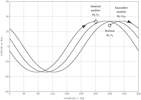
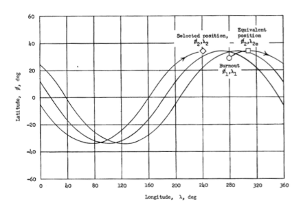
For comparison, here is her original diagram:

A more visually useful version can be constructed using GeoGraphics, taking care to convert the geocentric coordinates into geodetic coordinates:

path={#1,QuantityMagnitude[GeodesyData["Krassovsky",{"FromGeocentricLatitude",#2}]]}&@@@Flatten[points,1];

GeoGraphics[{Blue,PointSize[0.015],Point[GeoPosition[{ϕ1,λ1}]],Red,Point[GeoPosition[{ϕ2,λ2}]],Black,PointSize[0.002],Point[GeoPosition[Reverse/@path]]},GeoRange"World",GeoZoomLevel3]

How to Calculate Orbits Today

Today, virtually every one of us has, within immediate reach, access to computational resources far more powerful than those available to the entirety of NASA in the 1960s. Now, using only a desktop computer and the Wolfram Language, you can easily find direct numerical solutions to problems of orbital mechanics such as those posed to Katherine Johnson and her team. While perhaps less taxing of our ingenuity than older methods, the results one can get from these explorations are no less interesting or useful.

To solve for the azimuthal angle

using more modern methods, let's set up parameters for a simple circular orbit beginning after burnout over Florida, assuming a spherically symmetric Earth (I'll not bother trying to match the orbit of the Johnson paper precisely, and I’ll redefine certain quantities from above using the modern SI system of units). Starting from the same low-Earth orbit altitude used by Johnson, and using a little spherical trigonometry, it is straightforward to derive the initial conditions for our orbit:

ϕ1=28.50Degree(*latitudeofburnoutpoint*);λ1=(279.45-360)Degree(*longitudeofburnoutpoint*);

(*assumingacircularorbit,andleavingazimuthangleψundetermined*)r0=QuantityMagnitude[Quantity[21637933.,"Feet"],"Meters"](*radiusoftheorbit*);v0=Sqrt[GM/r0](*initialvelocityofthecircularorbit*);ℛ=RotationTransform[λ1,{0,0,1}](*usedtorotateinitialconditions*);{x0,y0,z0}=ℛ[{r0Cos[ϕ1],0,r0Sin[ϕ1]}](*initialx,y,zatburnoutpoint*);{vx0,vy0,vz0}=ℛ[v0{-Cos[ϕ1]Sin[γ]-Cos[γ]Cos[ψ]Sin[ϕ1],Cos[γ]Sin[ψ],Cos[γ]Cos[ϕ1]Cos[ψ]-Sin[γ]Sin[ϕ1]}](*initialvelocityattheburnoutpoint*);

initCond[ψ_,γ_]={x[0]==x0,y[0]==y0,z[0]==z0,x'[0]==vx0,y'[0]==vy0,z'[0]==vz0};

The relevant physical parameters can be obtained directly from within the Wolfram Language:

{M,R,G}=QuantityMagnitude[Flatten[{Entity["Planet","Earth"][{"Mass","Radius"}],Quantity[1,"GravitationalConstant"]}],"SIBase"];

Next, I obtain a differential equation for the motion of our spacecraft, given the gravitational field of the Earth. There are several ways you can model the gravitational potential near the Earth. Assuming a spherically symmetric planet and utilizing a Cartesian coordinate system throughout, the potential is merely:

pot[{x_,y_,z_}]:=-GM/Sqrt[x^2+y^2+z^2];

Alternatively, you can use a more realistic model of Earth’s gravity, where the planet’s shape is taken to be an oblate ellipsoid of revolution. The exact form of the potential from such an ellipsoid (assuming constant mass-density over ellipsoidal shells), though complicated (containing multiple elliptic integrals), is available through EntityValue:

evg=EntityValue

massive triaxial ellipsoid

PHYSICAL SYSTEM

,"GravitationalPotential";

For a general homogeneous triaxial ellipsoid, the potential contains piecewise functions:

(pw=Cases[evg,__Piecewise,∞][[1]])//TraditionalForm//Style[#,6]&

F -1 cos c a 2 a - 2 b 2 a - 2 c  2 a - 2 b - 2 x + 2 y  ( a - b )( a + b ) 2 a - 2 c + 2 c 2 y - 2 b 2 z a b c  2 b - 2 c  + E -1 cos c a 2 a - 2 b 2 a - 2 c  2 y - 2 z  2 a + 2 c  2 x - 2 y + 2 b  2 z - 2 x  ( a - b )( a + b ) 2 a - 2 c  2 c - 2 b 	2 x 2 a + 2 y 2 b + 2 z 2 c ≤1
F -1 sin 2 a - 2 c 2 a +κ 2 a - 2 b 2 a - 2 c  2 a - 2 b - 2 x + 2 y   2 a - 2 b  2 a - 2 c + E -1 sin 2 a - 2 c 2 a +κ 2 a - 2 b 2 a - 2 c  2 y - 2 z  2 a + 2 c  2 x - 2 y + 2 b  2 z - 2 x   2 a - 2 b  2 a - 2 c  2 c - 2 b  + - 2 c 2 y + 2 b 2 z +κ 2 z - 2 y   2 a +κ 2 b +κ 2 c +κ  2 c - 2 b 	True

Here, κ is the largest root of

+κ)+

(

+κ)+

+κ)1.

In the case of an oblate ellipsoid, the previous formula can be simplified to contain only elementary functions...

Limit[pw[[1,-1]],

]//FullSimplify

-2

ArcSin

κ+



κ+

(κ+

)

(κ+

)

+κ

-κ

(κ+

)

(κ+

)

-ArcSin

κ+



κ+

(

)(κ+

)

(κ+

)

-ArcSin

κ+



κ+

(

)(κ+

)

(κ+

)

+2ArcSin

κ+



κ+

ArcSin

κ+



κ+

(κ+

)

(κ+

)

+(κ+

)

+(-κ+

)

2

(

)

(κ+

)

(κ+

)



... where κ=



1/2

2



+

-



2

A simpler form that is widely used in the geographic and space science community, and that I will use here, is given by the so-called International Gravity Formula (IGF). The IGF takes into account differences from a spherically symmetric potential up to second order in spherical harmonics, and gives numerically indistinguishable results from the exact potential referenced previously. In terms of four measured geodetic parameters, the IGF potential can be defined as follows:

{a,b}=GeodesyData["ITRF00",#]&/@{"SemimajorAxis","SemiminorAxis"};gPole=9.8321849378(*gatEarth'spoleinm/s^2*);gEquator=9.78903267715(*gatEarth'sequatorinm/s^2*);With[{k=bgPole/(agEquator)-1,e=Sqrt[1-b^2/a^2]},potIGF[{x_,y_,z_}]:=With[{(*latitude*)ϕ=ArcTan[Sqrt[x^2+y^2],z]},-GM/Sqrt[x^2+y^2+z^2](1+kSin[ϕ]^2)/Sqrt[1-e^2Sin[ϕ]^2]]]

I could easily use even better values for the gravitational force through GeogravityModelData. For the starting position, the IGF potential deviates only 0.06% from a high-order approximation:

{potIGF[{x0,y0,z0}],GeogravityModelData[GeoPosition[GeoPositionXYZ[{x0,y0,z0}]],"Potential"]//QuantityMagnitude[#,"SIBase"]&}

{-6.04963×

,-6.05363×

}

With these functional forms for the potential, finding the orbital path amounts to taking a gradient of the potential to get the gravitational field vector and then applying Newton’s third law. Doing so, I obtain the orbital equations of motion for the two gravity models:

grad=-Grad[pot[{x[t],y[t],z[t]}],{x[t],y[t],z[t]}];gradIGF=-Grad[potIGF[{x[t],y[t],z[t]}],{x[t],y[t],z[t]}];

Fma={{x''[t],y''[t],z''[t]}grad};FmaIGF={{x''[t],y''[t],z''[t]}==gradIGF};

I am now ready to use the power of NDSolve to compute orbital trajectories. Before doing this, however, it will be nice to display the orbital path as a curve in three-dimensional space. To give these curves context, I will plot them over a texture map of the Earth’s surface, projected onto a sphere. Here I construct the desired graphics objects:

(*defineorbitburnoutDotandburnoutArrowgraphics*)burnoutCoords={x0,y0,z0};burnoutDirection={vx0,vy0,vz0}/v0;burnoutDot={Red,Sphere[burnoutCoords,R/30]};burnoutArrow={Red,Arrow[{burnoutCoords,burnoutCoords+(R/3)burnoutDirection}]};burnoutLabels[ψ_,γ_]=Graphics3D[{burnoutDot,burnoutArrow}];

(*defineglobetextureandmarkings*)earthTexture=Lighter[#,0.75]&@ImageReflect[PlanetData["Earth","CylindricalEquidistantTexture"],Bottom];globe=ParametricPlot3D[R{-Cos[p]Sin[t],-Sin[p]Sin[t],Cos[t]},{p,0,2Pi},{t,0,Pi},Mesh->None,PlotStyle->Texture[earthTexture],TextureCoordinateFunction->Automatic]

pole=Graphics3D[{Thick,Red,Line[{{0,0,-1.3R},{0,0,1.3R}}]}];equator=ParametricPlot3D[R{Cos[t],Sin[t],0},{t,0,2Pi},PlotStyleYellow];globeMarkings={pole,equator};

While the orbital path computed in an inertial frame forms a periodic closed curve, when you account for the rotation of the Earth, it will cause the spacecraft to pass over different points on the Earth’s surface during each subsequent revolution. I can visualize this effect by adding an additional rotation term to the solutions I obtain from NDSolve. Taking the number of orbital periods to be three (similar to John Glenn’s flight) for visualization purposes, I construct the following Manipulate to see how the orbital path is affected by the azimuthal launch angle ψ, similar to the study in Johnson’s paper. I’ll plot both a path assuming a spherical Earth (in white) and another path using the IGF (in green) to get a sense of the size of the oblateness effect (note that the divergence of the two paths increases with each orbit):

With[{ω=ωCapitale/(360/(2Pi)60),T=32Pir0/v0,ρ=Sqrt[x[t]^2+y[t]^2],ϕ=ArcTan[x[t],y[t]],γ=0.5Degree},Manipulate[Block[{ψ=ψs},sol=NDSolve[Join[Fma,initCond[ψs,γ]],{x,y,z},{t,0,τT}];solIGF=NDSolve[Join[FmaIGF,initCond[ψs,γ]],{x,y,z},{t,0,τT}];Show[ParametricPlot3D[Evaluate[{ρCos[ϕ-ωt],ρSin[ϕ-ωt],z[t]}/.{sol[[1]],solIGF[[1]]}],{t,0,τT},PlotStyle{White,Darker[Green]}]/.l_LineTube[l,35000],globe,globeMarkings,burnoutLabels[ψs,γ],FrameNone,TicksNone,PlotRange{All,All,{-1.2R,1.2R}},RotationAction"Clip",ViewPoint{0,-2,0.4}]],{{ψs,70Degree,"start angle"},-Pi,Pi},{{τ,1.025,"flight time"},0.001,3},SaveDefinitionsTrue]]

start angle

flight time

In the notebook attached to this blog, you can see this Manipulate in action, and note the speed at which each new solution is obtained. You would hope that Katherine Johnson and her colleagues at NASA would be impressed!

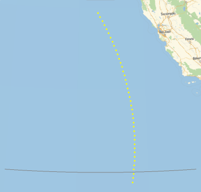
Now, varying the angle ψ at burnout time, it is straightforward to calculate the position of the spacecraft after, say, three revolutions:

posis=Block[{γ=0.5Degree,ω=ωCapitale/(360/(2Pi)60),T=3.052Pir0/v0},Table[Map[(Most[#]-{0,ωT360/(2Pi)})&,GeoPosition[GeoPositionXYZ[{x[T],y[T],z[T]}/.NDSolve[Join[FmaIGF,initCond[ψ,γ]],{x,y,z},{t,0,T}][[1]]]]],{ψ,50Degree,90Degree,1Degree}]];

GeoGraphics[{Gray,GeoPath[{"Parallel",28,{-135,-120}}],Yellow,Point[posis]},GeoRangeQuantity[450,"Miles"],GeoBackground"StreetMap",ImageSize400]

◼

Modeling the Reentry of a Satellite

The movie also mentions Euler’s method in connection with the reentry phase. After the initial problem of finding the azimuthal angle has been solved, as done in the previous sections, it’s time to come back to Earth. Rockets are fired to slow down the orbiting body, and a complex set of events happens as the craft transitions from the vacuum of space to an atmospheric environment. Changing atmospheric density, rapid deceleration and frictional heating all become important factors that must be taken into account in order to safely return the astronaut to Earth. Height, speed and acceleration as a function of time are all problems that need to be solved. This set of problems can be solved with Euler’s method, as done by Katherine Johnson, or by using the differential equation-solving functionality in the Wolfram Language.

For simple differential equations, one can get a detailed step-by-step solution with a specified quadrature method. An equivalent of Newton's famous

F=ma

for a time-dependent mass

m(t)

is the so-called ideal rocket equation (in one dimension)...

m(t)

′

(t)-

′

(t),

... where

m(t)

is the rocket mass,

the engine exhaust velocity and

′

(t)

the time derivative of the propellant mass. Assuming a constant

′

(t)

, the structure of the equation is relatively simple and easily solvable in closed form:

DSolve[{(m0-βt)v'[t]



β,v[0]vi},v[t],t]

{{v[t]vi+Log[m0]



-Log[m0-tβ]



}}

With initial and final conditions for the mass, I get the celebrated rocket equation (Tsiolkovsky 1903):

FormulaLookup["rocket equation"]

{RocketEquation}

FormulaData["RocketEquation"]

Log



FormulaData["RocketEquation","QuantityVariableTable"]

symbol	description	physical quantity	dimensions
v f	final speed	Speed	{{LengthUnit,1},{TimeUnit,-1}}
m f	final mass	Mass	{MassUnit,1}
m i	initial mass	Mass	{MassUnit,1}
v e	effective exhaust velocity	Speed	{{LengthUnit,1},{TimeUnit,-1}}
v i	initial speed	Speed	{{LengthUnit,1},{TimeUnit,-1}}

FormulaData@FormulaLookup["rocket equation"][[1]]

Log



The details of solving this equation with concrete parameter values and e.g. with the classical Euler method I can get from Wolfram|Alpha. Here are those details together with a detailed comparison with the exact solution, as well as with other numerical integration methods:

WolframAlpha["use Euler method (2-t)v'(t)=4, v(0)=0, from t=0 to 0.95"]

Input interpretation

solve

(2-t)

′

(t)4

v(0)0

using Euler method

from t  0 to 0.95

Solution plot

Hide error plot

	exact result
	numerical solution

Error plot

(using 10 steps with stepsize 0.095)

Stepwise results

step	t	v	local error	global error
0	0.	0.	0	0
⋮	⋮	⋮	⋮	⋮
10	0.95	2.49345	-0.0335421	0.0839779

+ Definitions

Butcher tableau

1
	1

Symbolic iteration code

′

(t)f(t,v)4, v(0)0

n + 1



+ h

n + 1



+ h

f(

)

f(

+ h,

+ h

)

where v 0 	0
t 0 	0
h 	0.095
n 	0,…,10

Stability region in complex stepsize plane

stability function: z+1

Exact solution of equation

v(t)  4(-log(t-2)+π+log(2))

log(x) is the natural logarithm

Stepsize comparison

(global error at t  0.95)

Method comparison

method	global error	log scale comparison
forward Euler method	0.0840
midpoint method	0.000986
Heun's method	0.0000232
third-order Runge-Kutta method	-5.13× -7 10
fourth-order Runge-Kutta method	-5.13× -7 10
Runge-Kutta-Fehlberg method	4.19× -8 10
Bogacki-Shampine method	4.28× -9 10
Dormand-Prince method	6.31× -10 10
backward Euler method	-0.0879
implicit midpoint method	0.000986

(global error at t  0.95using 10 steps with stepsize 0.095)

Mathematica input

NDSolve[{(2 - t) v'[t] == 4, v[0] == 0}, v, {t, 0, 0.95}, Method-> {"FixedStep", Method -> "ExplicitEuler"}, StartingStepSize -> 0.095, WorkingPrecision -> MachinePrecision]

Following the movie plot, I will now implement a minimalistic ODE model of the reentry process. I start by defining parameters that mimic Glenn's flight:

(*Glenn'sflight*)mCapsule=QuantityMagnitude

Mercury Atlas 6

MANNED SPACE MISSION



mass

,"SIBase";(*massofMercuryAtlas6*)ϕ0=34.00;λ0=241.00Degree;(*initiallatitudeandlongitude*)h=QuantityMagnitude

Mercury Atlas 6

SATELLITE



average altitude

,"Meters";

X0=(R+h){Cos[λ0]Cos[ϕ0],Sin[λ0]Cos[ϕ0],Sin[ϕ0]};(*positionatstartofreentry*)V0=Sqrt[GM/(R+h)]{-Sin[λ0],Cos[λ0],0};(*velocityatstartofreentry*)

I assume that the braking process uses 1% of the thrust of the stage-one engine and runs, say, for 60 seconds. The equation of motion is:

caps

′

(t)

grav

(x(t))+

exhaust

(t)+

friction

(x(t),v(t))

Here,

grav

is the gravitational force,

exhaust

(t)

the explicitly time-dependent engine force and

friction

(x(t),v(t))

the friction force. The latter depends via the air density explicitly on the position

x(t)

and via the friction law on

v(t)

For the height-dependent air density, I can conveniently use the StandardAtmosphereData function. I also account for a height-dependent area because of the parachute that opened about 8.5 km above ground:

Cd=1(*dragcoefficient*);airDensity[X:{_Real,__}]:=QuantityMagnitude[StandardAtmosphereData[Quantity[Norm[X]-R,"Meters"],"Density"],"SIBase"]airFriction[X_List,V_List]:=-1/2area[Norm[X-R]]V.VCdairDensity[X]V/Sqrt[V.V]brake[V_List,t_,{α_,T_}]:=-If[t<T,αNormalize[V],0]

This gives the following set of coupled nonlinear differential equations to be solved. The last WhenEvent[…] specifies to end the integration when the capsule reaches the surface of the Earth. I use vector-valued position and velocity variables X and V:

area[height_]:=If[h>8500,10,(*parachute*)2000];

With these definitions for the weight, exhaust and air friction force terms...

Fgrav[X_,V_,t_]:=-GmCapsuleMX/Sqrt[X.X]^3Fexhaust[X_,V_,t_]:=brake[V,t,{3000,60}]Fairfraction[X_,V_,t_]:=airFriction[X,V]

... total force can be found via:

Ftotal[X_,V_,t_]:=Fgrav[X,V,t]+Fexhaust[X,V,t]+Fairfraction[X,V,t]

odeSystem={X'[t]V[t],mCapsuleV'[t]Ftotal[X[t],V[t],t],WhenEvent[Norm[X[t]]-R0,"StopIntegration"]};

In this simple model, I neglected the Earth’s rotation, intrinsic rotations of the capsule, active flight angle changes, supersonic effects on the friction force and more. The explicit form of the differential equations in coordinate components is the following. The equations that Katherine Johnson solved would have been quite similar to these:

(odeSystem/.{X({x[#],y[#],z[#]}&),V({vx[#],vy[#],vz[#]}&)}/.w_WhenEvent:>Evaluate//@w)//Column[#,DividersCenter]&

{

′

[t],

′

[t],

′

[t]}{vx[t],vy[t],vz[t]}

{1352.0

′

[t],1352.0

′

[t],1352.0

′

[t]}-If[t<60,3000Normalize[{vx[t],vy[t],vz[t]}],0]-5airDensity[{x[t],y[t],z[t]}]vx[t]

vx[t]

vy[t]

vz[t]

5.389×

x[t]

3/2

(

x[t]

y[t]

z[t]

)

,-If[t<60,3000Normalize[{vx[t],vy[t],vz[t]}],0]-5airDensity[{x[t],y[t],z[t]}]vy[t]

vx[t]

vy[t]

vz[t]

5.389×

y[t]

3/2

(

x[t]

y[t]

z[t]

)

,-If[t<60,3000Normalize[{vx[t],vy[t],vz[t]}],0]-5airDensity[{x[t],y[t],z[t]}]vz[t]

vx[t]

vy[t]

vz[t]

5.389×

z[t]

3/2

(

x[t]

y[t]

z[t]

)



WhenEvent-6.3710088×

Abs[x[t]]

Abs[y[t]]

Abs[z[t]]

0,StopIntegration

Supplemented by the initial position and velocity, it is straightforward to solve this system of equations numerically. Today, this is just a simple call to NDSolve. I don’t have to worry about the method to use, step size control, error control and more because the Wolfram Language automatically chooses values that guarantee meaningful results:

tMax=5000;inits={X[0]X0,V[0]V0};nds=NDSolve[Join[odeSystem,inits],{X,V},{t,0,60,tMax}]

X

InterpolatingFunction



Domain: {{0.,1440.}}

Output dimensions: {3}



,V

InterpolatingFunction



Domain: {{0.,1440.}}

Output dimensions: {3}





Here is a plot of the height, speed and acceleration as a function of time:

plotXVAT[nds_]:=With[{T=nds[[1,1,2,1,1,2]]/60,opts=Sequence[ImageSize220,PlotRangeAll]},GraphicsRow[{Plot[(Norm[X[60t]]-R)/1000/.nds[[1]],{t,0,T},opts,AxesLabel{"time (min)","height (km)"}],Plot[Norm[V[60t]]/1000/.nds[[1]],{t,0,T},opts,AxesLabel{"time (min)","speed (km/s)"}],Plot[Norm[Ftotal[X[60t],V[60t],60t]]/(9.81mCapsule)/.nds[[1]],{t,0,T},opts,AxesLabel{"time (min)","acceleration (g)"}]},Spacings0]]

plotXVAT[nds]

Plotting as a function of height instead of time shows that the exponential increase of air density is responsible for the high deceleration. This is not due to the parachute, which happens at a relatively low altitude. The peak deceleration happens at a very high altitude as the capsule goes from a vacuum to an atmospheric environment very quickly:

With[{T=nds[[1,1,2,1,1,2]]/60,opts=Sequence[ImageSize220,PlotRangeAll]},ParametricPlot[Evaluate[{(Norm[X[60t]]-R)/1000,Norm[Ftotal[X[60t],V[60t],60t]]/(9.81mCapsule)}/.nds[[1]]],{t,0,T},opts,AxesLabel{"height (km)","acceleration (g)"},AspectRatio0.6]]

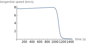
And here is a plot of the vertical and tangential speed of the capsule in the reentry process:

With[{T=nds[[1,1,2,1,1,2]],opts=Sequence[ImageSize300,PlotRangeAll]},{Plot[V[t].Normalize[X[t]]/1000/.nds[[1]],{t,0,T},opts,AxesLabel{"time (s)","vertical speed (km/s)"}],Plot[(Norm[V[t]-V[t].Normalize[X[t]]Normalize[V[t]]])/1000/.nds[[1]],{t,0,T},opts,AxesLabel{"time (s)","tangential speed (km/s)"}]}]





Now I repeat the numerical solution with a fixed-step Euler method:

ndsEuler=NDSolve[Join[odeSystem,inits],{X,V},{t,0,tMax},Method{"FixedStep",Method"ExplicitEuler"},StartingStepSize0.05]

X

InterpolatingFunction



Domain: 0.,1.44×



Output dimensions: {3}



,V

InterpolatingFunction



Domain: 0.,1.44×



Output dimensions: {3}





Qualitatively, the solution looks the same as the previous one:

plotXVAT[ndsEuler]

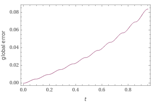
For the used step size of the time integration, the accumulated error is on the order of a few percent. Smaller step sizes would reduce the error (see the previous Wolfram|Alpha output):

With[{T=nds[[1,1,2,1,1,2]]},Plot[100((Norm[X[t]]-R/.nds[[1]])/(Norm[X[t]]-R/.ndsEuler[[1]])-1),{t,0,T},AxesLabel{"time (s)","height error (%)"}]]

Note that the landing time predicted by the Euler method deviates only 0.11% from the previous time. (For comparison, if I were to solve the equation with two modern methods, say "BDF" vs. "Adams", the error would be smaller by a few orders of magnitude.)

Now, the reentry process generates a lot of heat. This is where the heat shield is needed. At which height is the most heat per area

generated? Without a detailed derivation, I can, from purely dimensional grounds, conjecture



~ρ

DimensionalCombinations[{"Speed","MassDensity"},"HeatFlux"]

{

MassDensity

Speed

}

With[{T=nds[[1,1,2,1,1,2]]},ParametricPlot[Evaluate[{(Norm[X[t]]-R)/1000,airDensity[X[t]]Norm[V[t]]^3}/.nds[[1]]],{t,0,T},PlotRangeAll,Ticks{True,False},AxesLabel{"height (km)","heat generated (a.u.)"},AspectRatio0.6]]

Many more interesting things could be calculated (Hicks 2009), but just like the movie had to fit everything into two hours and seven minutes, I will now end my blog for the sake of time. I hope I can be pardoned for the statement that, with the Wolfram Language, the sky’s the limit.

Cite this as: Jeffrey Bryant, "Hidden Figures: Modern Approaches to Orbit and Reentry Calculations" from the Notebook Archive (2017), https://notebookarchive.org/2018-07-6xhkzoc

​​Hidden Figures: Modern Approaches to Orbit and Reentry Calculations

Constants and Initial Processing

Computation

Plotting

How to Calculate Orbits Today

Hidden Figures: Modern Approaches to Orbit and Reentry Calculations