Holistic Mathematics, vol. 1
Author
John Erickson
Title
Holistic Mathematics, vol. 1
Description
We us a recreational discrete math problem to explore issues in math and math education.
Category
Educational Materials
Keywords
math, recreational math, discrete math, math education
URL
http://www.notebookarchive.org/2021-01-5kgfmyo/
DOI
https://notebookarchive.org/2021-01-5kgfmyo
Date Added
2021-01-12
Date Last Modified
2021-01-12
File Size
1.61 megabytes
Supplements
Rights
CC BY-NC-SA 4.0

Holistic Mathematics: Experiments, Computation, and Proof: Vol 1
Holistic Mathematics: Experiments, Computation, and Proof: Vol 1
John Erickson, PhD
“Think deeply about simple things.” -Arnold Ross
“Everyone has a book inside them, which is exactly where it should, I think, in most cases, remain.” -Christopher Hitchens
Mathematicians always strive to confuse their audiences; where there is no confusion there is no prestige. Mathematics is prestidigitation. -Carl E. Linderholm Mathematics Made Difficult

Prologue to all 4 volumes (abridged)
Prologue to all 4 volumes (abridged)
This monograph is a bit weird, but maybe it’s time for a little weird because normal and conventional has clearly not worked out so well when it comes to some of the problems in math education in my opinion.
There are several goals for this four volume monograph. Too many times students have asked me “How do you do research in mathematics?” and I have found that the best way, perhaps the only way, is to just do some research with them. Since that isn’t a scalable solution, my main goal is to illustrate, at a fairly elementary level, one approach to how math research can be done by providing a concrete and comprehensive, albeit vicarious, research experience which goes “from grammar school to graduate school”. I put that in quotes because I thought I made it up, but I’m apparently not the only one who says this. In order to facilitate this goal, I have sort of “let it all hang out” so to speak, nothing gross mind you, I just haven’t removed all the evidence of work, false approaches, incorrect ideas, and shortcomings. This gives the monograph a rough quality, but that is not intended as an excuse for actual mistakes, of which I am sure there are many.
The problem which started our investigation was an essentially randomly chosen elementary recreational discrete math problem. Someone sent me their kids math circle problem. Now, I make no claim to being a great mathematician and, in particular, I am not really all that great at discrete mathematics. Contrary to this being a deficit however, this was actually an advantage for my goals, since an expert would likely know the standard machinery and be done with it. I, on the hand, actually had to think about the problem and create some code to make sure I understood what was going on. After solving the problem I decided I would see what would happen if I just followed the mathematics to see where it led through the standard process of both generalization and specialization. In the end, I would say that the journey wound up being a seemingly random “stop and smell the roses” tour of mathematics. Speaking of the “end”, my stopping criteria, that I end up at the graduate level, was a bit problematic since it took about three years and perhaps I only ended up at the advanced undergraduate beginning graduate student level. If you’re the sort that likes to know where you are going before you begin a journey, the last result, in volume 4, is from computational and theoretical combinatorial group theory. Alexander Hulpke and I added sequence A337015 to the OEIS and proved a nice but simple theorem connecting sequences A005432 and A337015 which makes one ask how else these sequences might be related. One question I find interesting to ask is the following: if I started with the exact same problem today would I end up three years later arriving at the same terminal result or not?
Just to be absolutely clear, there is really nothing original in my approach, which is probably most influenced by Polya, Ross, and even Moore (sans all of his racism) along with various teachers and professors I have had. I would say that it is also heavily influenced by my modest knowledge of experimental mathematics and the use of software to do calculations. I used Mathematica primarily along with the OEIS, but I also used WolframAlpha, the Inverse Symbolic Calculator, and GAP as well. There are many choices for tools and the underlying mathematics does not depend on those choices. Here is an interesting related issue regarding the balance of math and computation. I have noticed that a lot of students who like coding neglect math these days, and would be quite happy if they never saw another equation again. I find this situation unfortunate. On the other hand, I have also been told by well meaning, and very smart math people, that I should remove or otherwise segregate all the code in these volumes. I said to myself, “Yeah, that ain’t ever gonna happen.” Am I in love with my own code and just being stubborn you ask? I don’t think so. Obviously, I think learning to code is important, but the primary reason I have left the code in place is that I am firmly convinced that the tendency to present the slick final product of our mathematical labors in the form of an elegant proof without the motivations, experiments, and even incorrect understandings, is part of the reason so many students turn away from mathematics. They say to themselves, “Well, I could never do that, I better switch majors.” This is particularly true for students who are already insecure, in particular, members of underrepresented groups.
The basic process we will follow throughout the volumes is simple, and is what mathematicians do all the time: play with some mathematical problem, consider examples, run experiments, look at visualizations, notice patterns, make conjectures and try to prove them. Inevitably, you will make new definitions and generalizations and find new patterns, make new conjectures, prove new theorems, etc...Eventually you may find that you are able to make conjectures that you can’t prove. That could be because they are not true, or you simply don’t have the background knowledge needed, and that’s fine, albeit a bit frustrating.
Another goal of this monograph to constructively criticize some trends in math education which I find deeply problematic. Basically, while I believe that lists of best teaching practices can be productively adapted by each individual instructor for their particular students, some of the confidently asserted alleged universal “research driven best practices” for teaching mathematics sound rather dubious to me and perhaps even counter productive. I will at times freely just be giving my opinions based on my own training and experiences as a student, as a high school teacher, as a community college instructor and as a college professor. They are just my opinions, so please feel free to disagree. In particular, I will also occasionally address all the endless talk about the importance of diversity and the reality of “uhh...yeah, not so much”. I finally concluded that it was my duty to address some of these issues, and it was cheaper than paying for therapy. For people who want to read the math or code, but don’t want to read this material, I get it, nobody wants to feel uncomfortable. Therefore, I have helpfully delineated these comments with the word Comment.
Finally, since the primary target audience for this monograph was students, now and in the future, it was important to me that I leave the comments in place and that the book be as cheap as possible. Having said that, faculty that have an interest in teaching or how ideas are arrived at, might find this interesting as well.
Disclaimers & Comments
Disclaimers & Comments
◼
The opinions expressed in this document are mine and mine alone and do not represent the opinions nor constitute an endorsement of/by any other person or entity mentioned in this monograph. If your name was mentioned it was simply to properly acknowledge precedence or give credit.
◼
This is a first iteration. In addition to not having been vetted mathematically, I couldn’t talk my wife into proofreading it once she heard it was four volumes, so the writing is what it is. If she had helped me, she could have removed this statement.
◼
No claim is being made regarding the originality or importance of the results presented in this monograph. Obviously, it would have been nice if we had stumbled onto a slick proof of the Riemann Hypothesis, but that didn’t happen. I’m telling myself that It’s more about the process than the results.
◼
No claim is being made regarding the optimality of the code.
◼
Regarding the poor layout, I never figured out how to use Mathematica stylesheets or the author tools, but I intend to ask Wolfram Research for help with this in a future iteration.
Preface to Vol 1
Preface to Vol 1
We introduce a problem called the last one standing problem which started us off and is about binary sequences. We then abstract and reframe the problem in terms of permutations. We will think about various ways to generate the sequence automatically and this will get us thinking more about coding. Explaining why the code is doing what it is supposed to be doing will require mathematics. Along the way we will be producing sequences of integers and this is where the OEIS will play a role as we try to conjecture formulas for the sequences and ultimately prove them. We will also endeavor to connect the concrete and the abstract and finally make some connections with other parts of mathematics.
Chapter 1-The Initial Problem
We introduce the problem that started this all off.
The Problem
The Problem
The problem we will initially investigate is called the last one standing problem. It is stated as follows:
n
n-1
◼
A student may switch between sitting and standing only if the student immediately to it’s left is standing and all the students further left are sitting.
◼
The farthest left student can switch at will.
◼
The status of students to the right don’t matter.
How many steps does it take to solve the problem in an optimal solution?
Clearly, we don’t need actual students to solve this problem and we can use 1’s and 0’s or “black” and “white” as substitutes for standing and sitting according the to the correspondence
|
Despite its elementary nature, I am slightly embarrassed to say that I had actually never heard of it. However, as is often the case when you “think deeply about simple things” it turns out to be pretty interesting. Before tackling the problem at hand a few questions are in order. Mathematicians are trained to automatically ask questions that most people would take for granted.
Question 1
Question 1
The first question we should ask, and the only one we will answer immediately, is “does a solution exist at all?!” How do you know you can get to {0,0,0,1} using these rules?
The answer to this question is easy since we can simply manually compute a solution as follows.
In[]:=
array={{0,0,0,0},{1,0,0,0},{1,1,0,0},{0,1,0,0},{0,1,1,0},{1,1,1,0},{1,0,1,0},{0,0,1,0},{0,0,1,1},{1,0,1,1},{1,1,1,1},{0,1,1,1},{0,1,0,1},{1,1,0,1},{1,0,0,1},{0,0,0,1}};
We can make the steps look nicer as follows
Grid[array]
0 | 0 | 0 | 0 |
1 | 0 | 0 | 0 |
1 | 1 | 0 | 0 |
0 | 1 | 0 | 0 |
0 | 1 | 1 | 0 |
1 | 1 | 1 | 0 |
1 | 0 | 1 | 0 |
0 | 0 | 1 | 0 |
0 | 0 | 1 | 1 |
1 | 0 | 1 | 1 |
1 | 1 | 1 | 1 |
0 | 1 | 1 | 1 |
0 | 1 | 0 | 1 |
1 | 1 | 0 | 1 |
1 | 0 | 0 | 1 |
0 | 0 | 0 | 1 |
We can actually easily make a simple visualization as well in which black is 1 or standing and white is 0 or sitting.
In[]:=
Clear[p]
In[]:=
Out[]=
|  | ||||||
|

The problem is that we have no insight into what is going on with just one manual calculation which leads to some additional questions.
Question 2
Question 2
Can we always solve the last one standing problem for an arbitrary number, , of people? Using these rules, which other binary n-digit sequences are reachable?
n
Question 3
Question 3
A manual calculation is fine for but what about or more? Is there a way to automate the solution?
n=4
n=10
Question 4
Question 4
Is there a “natural” order preserving correspondence between the sequences in the steps of a solution and the set of positive integers {1,2,3,..., } where is the number of sequences in a solution.
m
m
Two Solutions to our initial Problem
Two Solutions to our initial Problem
There are several ways to approach this problem, perhaps even many, but we will focus on two for now and our approach will be informal initially.
Solution 1
Solution 1
Our first solution is essentially an inductive one in which we relate the number of steps in a solution to the case to the number of steps in the case. It is interesting that this was my first solution, as it is not the simplest, but I think it was because the problem was stated in terms of “steps” and the parent who sent the original email had provided the above explicit solution to the case in the form of a spreadsheet in which they had segregated the first row of {0,0,0,0} by itself, thereby “breaking the symmetry” of the solution sequence.
th
n
n-
st
1
n=4
We create a manipulate to more easily visualize the solution. The first blue horizontal line is only meant to segregate the first row since we are counting steps instead of rows.
In[]:=
Manipulate[Grid[array,Background{None,None,{{{1,},{1,n}}LightRed}},Dividers{{nBlue},{2Blue,+1Blue,+2Blue}}],{n,{1,2,3,4}},SaveDefinitionsTrue]
n
2
n-1
2
n-1
2
Out[]=
| | ||||||||||||||||||||||||||||||||||||||||||||||||||||||||||||||||||||||||
| |||||||||||||||||||||||||||||||||||||||||||||||||||||||||||||||||||||||||
Anytime we encounter a problem like this, it helps to experiment with small cases. It is clear that if one person is sitting, it takes them 1 move to stand as they are furthest to the left (trivially) and can stand at will. If two people are sitting it is pretty clear that it will take 3 moves. The picture above isn’t really necessary to see this and the additional lines needlessly complicate things actually. For however we can see a pattern emerge. We can see from the above picture that it takes 7 moves if . Let’s just take this for granted for the moment and now consider or the {0,0,0,0} initial state. If we only look at the first 3 positions we can see that it takes 7 moves to get to {0,0,1,0}. Then we use our rule and make one move to change the last 0 to a 1 and get {0,0,1,1}. Now we see that it takes another 7 moves to get to {0,0,0,1}. This makes sense since we may now focus on the first 3 digits and instead of {0,0,0} to {0,0,1} we are going from {0,0,1} to {0,0,0}. Intuitively, these should be the same since we just have to reverse our steps.
n=3or4
n=3
n=4
More precisely, in the language of recurrence relations, if we let be the number of moves for people we have that =+1+ which gives =2+1. Also, =1.
t
n
n
t
n
t
n-1
t
n-1
t
n
t
n-1
t
1
Clear[t]
t[1]=1;t[n_]:=2t[n-1]+1;
Table[{k,t[k]},{k,1,10}]//TableForm
1 | 1 |
2 | 3 |
3 | 7 |
4 | 15 |
5 | 31 |
6 | 63 |
7 | 127 |
8 | 255 |
9 | 511 |
10 | 1023 |
If you look at these numbers long enough you can guess that =-1. This formula can be proved by induction or you can could just solve for an explicit solution using Mathematica.
t
n
n
2
Clear[t];RSolve[{t[n]==2t[n-1]+1,t[1]1},t[n],n][[1]]//TraditionalForm
{t(n)-1}
n
2
If you don’t have Mathematica, you can just type “solve t(1)=1; t(n)=2 t(n-1)+1”, without the quotes, into WolframAlpha.
This is the same recurrence, and therefore the same solution, as in the famous “Tower of Hanoi” problem. In fact, I just copied most of this section from some notes I gave my former students for the tower of Hanoi problem. This suggests that there may be a way to solve the last one standing problem by “mapping” it to the tower of Hanoi problem. In addition to having the same move count, the clue that the last one standing problem can probably be connected to the tower of Hanoi problem is that in the tower of Hanoi problem, you also complete about half the task of moving the disks by first moving the top disks to the middle peg, then you move the largest disk to the last peg, and finally we move the smaller disks from the middle peg on top of the largest disk. The structural similarity to what we have described above is too close to be a coincidence. Despite this interesting connection, we don’t pursue this line of thinking any further as we want to take the last one standing problem on its own merits and, frankly, off hand, we don’t see how it can really help us since we don’t know anything more about the Tower of Hanoi problem and its solution than is contained in the above discussion.
n
n-1
n-1
Finally, it has recently been brought to my attention that the famous Chinese rings puzzle (which I didn’t know about) is yet another mathematical recreational problem related to the last one standing problem. This puzzle apparently has the advantage of enforcing the correct “move” at each step rather than merely exhorting the player to use as few moves as possible.
A “by hand” solution to the recurrence
A “by hand” solution to the recurrence
Of course, there are methods to solve these types of recurrence relation problems by hand as well and for some people it is satisfying to know that this is not something that only a computer can understand, so we mention it briefly.
To solve =2+1 we first solve the homogeneous problem -2=0. The solution is obviously =α, but we could solve this using the characteristic equation . It turns out that there is a general theory of linear recurrence relations which tells us that the general solution is of the form =α+β. Now we know that =1 and =3. Therefore we have and . It is easy to show that these equations imply orα=1 so that we may now conclude that giving us a final solution of =-1 as we said.
t
n
t
n-1
t
n
t
n-1
t
n
n
2
r-2=0
t
n
n
2
t
1
t
2
1=2α+β
3=4α+β
2α=2
β=-1
t
n
n
2
Solution 2
Solution 2
The key idea in this solution is to realize that instead of counting the steps, as the problems asks, just count the number of binary sequences and subtract 1. Counting the steps “breaks the symmetry” of the problem, thereby making things more cumbersome. Incidentally, symmetry will play a large role in this entire monograph which is only fitting since it plays a large role in mathematics in general. We can make a simple manipulate, which clearly shows the symmetry of the problem and how to relate the number of binary sequences in the case to the number of binary sequences in the case.
th
n
n-
st
1
Again, we create a manipulate to visualize the problem.
In[]:=
Manipulate[Grid[array,Background{None,None,{{{1,},{1,n}}LightRed}},Dividers{{nBlue},{+1Blue}}],{n,{1,2,3,4}},SaveDefinitionsTrue]
n
2
n-1
2
Out[]=
| | ||||||||||||||||||||||||||||||||||||||||||||||||||||||||||||||||||||||||
| |||||||||||||||||||||||||||||||||||||||||||||||||||||||||||||||||||||||||
The picture above clearly shows that we are simply doubling the number of sequences as we add an additional digit! The horizontal blue line in the diagram simply acts a mirror line of symmetry for the digit sequences to the left of the vertical blue line. Moreover, it is now clear that the number of sequences required to transform {0,0,...,0,0} to {0,0,...,1,0} is the same as the numbers of sequences required to transform {0,0,...,1,1} to {0,0,...,0,1} since you simply to do the reverse of what you did to transform {0,0,...,0,0} to {0,0,...,1,0}.
More precisely, in the language of recurrence relations, if we let be the number of sequences for digits we have that =+ which gives =2. Also, =2. The solution to this recurrence is clearly =, without having to do anything fancy with a computer or by hand, and the number of steps will be -1 so we have answered the main and initial question. Technically, one could make a mountain out of a mole hill and do a “proof by induction” but that seems gratuitous here.
s
n
n
s
n
s
n-1
s
n-1
s
n
s
n-1
s
1
s
n
n
2
n
2
Some Observations, Patterns, and Visualizations
Some Observations, Patterns, and Visualizations
Evidently the rules specified for this problem have produced a sequence of positions with lots of patterns and symmetry. It is these symmetrical patterns that we will use to solve the problem. Patterns are a common theme of mathematics and may in fact comprise the essence and very definition of mathematics.
Perhaps you have noticed that something a little strange is going on with our current pattern: since our solution appears to be generating distinct sequences, we are simply getting all possible binary sequences and there really was no a priori reason for this to occur.
n
2
n
2
In base 2 we can write the 16 numbers from 0 to 15 base 10 as follows:
Table[BaseForm[k,2],{k,0,15}]
{,,,,,,,,,,,,,,,}
0
2
1
2
10
2
11
2
100
2
101
2
110
2
111
2
1000
2
1001
2
1010
2
1011
2
1100
2
1101
2
1110
2
1111
2
If we use 0 as a place holder, we can list out all 16 4-digit binary numbers can be listed as follows:
Tuples[{0,1},4]
{{0,0,0,0},{0,0,0,1},{0,0,1,0},{0,0,1,1},{0,1,0,0},{0,1,0,1},{0,1,1,0},{0,1,1,1},{1,0,0,0},{1,0,0,1},{1,0,1,0},{1,0,1,1},{1,1,0,0},{1,1,0,1},{1,1,1,0},{1,1,1,1}}
Since we have 4 slots and 2 choices for each slot we expect =16 sequences.
4
2
So we can see that our solution array is nothing more than a rearrangement or permutation of all 16 four digit binary numbers, which, again, begs the question: why does our rule run through all possible 4 digit binary sequences? There are probably many ways to think about this. One way to see that we get 16 unique sequences is to argue that we have 4 slots into which we can either choose to put a 0 or a 1 and each sequence represents a unique sequence of choices. We can actually see this if we change our perspective and flip the table. From this point of view it is clear that our list of sequences has a tree structure.
Grid[Transpose[Reverse/@array]]
0 | 0 | 0 | 0 | 0 | 0 | 0 | 0 | 1 | 1 | 1 | 1 | 1 | 1 | 1 | 1 |
0 | 0 | 0 | 0 | 1 | 1 | 1 | 1 | 1 | 1 | 1 | 1 | 0 | 0 | 0 | 0 |
0 | 0 | 1 | 1 | 1 | 1 | 0 | 0 | 0 | 0 | 1 | 1 | 1 | 1 | 0 | 0 |
0 | 1 | 1 | 0 | 0 | 1 | 1 | 0 | 0 | 1 | 1 | 0 | 0 | 1 | 1 | 0 |
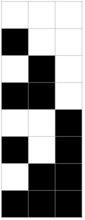
We can make the tree structure even more visible by wrapping the above in ArrayPlot. Black is 1 and white is 0.
In[]:=
ArrayPlot[Transpose[Reverse/@array],AspectRatio1,MeshTrue,ImageSizeSmall]
Out[]=

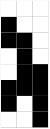
Notice that while the above has a tree structure but it looks different than the tree structure below which could be described as white is left and black is right.
In[]:=
ArrayPlot[Transpose[Tuples[{0,1},4]],AspectRatio1,MeshTrue,ImageSizeSmall]
Out[]=

Of course, we can create an actual tree in Mathematica easily as follows.
CompleteKaryTree[5]

Notice that we have actually answered, at an intuitive level, questions 1 and 2 asked above: yes, for any , we can always reach the {0,0,....,0,1} sequence and, in fact, any sequence, since we go through all sequences.
n
n
2
How to construct the list programmatically
How to construct the list programmatically
Using our observations of patterns and symmetries in the previous sections, we can construct solutions to the last one standing problem programmatically. There are many ways to do this and in this section we will show two related approaches. Are we doing math or computer science in this section you ask? Yes! These naming distinctions are not precise terms nor even really all that important, but they do serve to provide a rough idea of an area of interest. It’s true that focusing on how to construct an object algorithmically, rather than merely proving that an object exists, comes up in computer science, but algorithms in mathematics predate the invention of computers by millennia (think Euclid’s algorithm on the computation of the GCD for example). Of course, we are happy that we have a computer to implement our algorithms, and the Wolfram language in particular makes these sorts of tasks fairly easy once you get the hang of it. Obviously, you can do these implementations in whatever language you like.
We won’t go into great detail as to how these methods work as it is your task to figure out the details and part of the objective in this section is simply to expose you to different ways to program in the Wolfram language.
Method 1
Method 1
First we construct an auxiliary function which takes a list, adds a 0 at the end to all the elements in the list, then adds a 1 to the end of all the elements of the list and reverses the resulting list. Finally, this function joins both lists.
In[]:=
lastOneStandingFunction[x_]:=Join[Append[#,0]&/@x,Reverse[Append[#,1]&/@x]];
For example if we have {{0,0},{1,0},{1,1},{0,1}} as our input list we get the following
lastOneStandingFunction[{{0,0},{1,0},{1,1},{0,1}}]
{{0,0,0},{1,0,0},{1,1,0},{0,1,0},{0,1,1},{1,1,1},{1,0,1},{0,0,1}}
Using this function we can now generate our solution to the last one standing problem programmatically by using Nest with the lastOneStandingFunction.
In[]:=
Manipulate[Grid[Nest[lastOneStandingFunction,{{0},{1}},n-1]],{n,{1,2,3,4,5}},SaveDefinitionsTrue]
Out[]=
| | |||||||||||||||||||||||||||||||||
| ||||||||||||||||||||||||||||||||||
It should be clear yet again now why the number of sequences is doubling since we are joining lists of identical lengths.
We can use ArrayPlot in place of Grid to get a nice vertical visualization of the array.
In[]:=
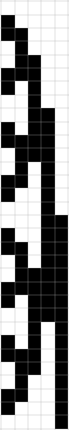
Manipulate[ArrayPlot[Nest[lastOneStandingFunction,{{0},{1}},n-1],MeshTrue,ImageSizeSmall],{n,{1,2,3,4,5}},SaveDefinitionsTrue]
Out[]=
| | |||||||||
| ||||||||||
Method 2
Method 2
In a previous section, with , we noticed that our sequence was a re-ordering of the binary digits of the numbers 0 to 15 but exactly what re-ordering of the digits 0 though 15 is this? First we convert to base 10.
n=4
FromDigits[#,2]&/@{{0,0,0,0},{1,0,0,0},{1,1,0,0},{0,1,0,0},{0,1,1,0},{1,1,1,0},{1,0,1,0},{0,0,1,0},{0,0,1,1},{1,0,1,1},{1,1,1,1},{0,1,1,1},{0,1,0,1},{1,1,0,1},{1,0,0,1},{0,0,0,1}}
{0,8,12,4,6,14,10,2,3,11,15,7,5,13,9,1}
If you stare at this list long enough you can see a pattern, but figuring out exactly how to generate this list with just decimal operations is a little bit tricky. Once we know how to generate this list it will however be a simple matter to recover the array we desire as follows:
IntegerDigits[#,2,4]&/@{0,8,12,4,6,14,10,2,3,11,15,7,5,13,9,1}
{{0,0,0,0},{1,0,0,0},{1,1,0,0},{0,1,0,0},{0,1,1,0},{1,1,1,0},{1,0,1,0},{0,0,1,0},{0,0,1,1},{1,0,1,1},{1,1,1,1},{0,1,1,1},{0,1,0,1},{1,1,0,1},{1,0,0,1},{0,0,0,1}}
Having stared at the list of decimal numbers you will eventually notice that if you divide it in half, the second half entries are just one more than the first half entries in reverse. Moreover, the first half entries are all even. That’s a lot of words to say that this list is generated by iterating the operation of . Again, the Nest command is often useful to implement recursive solutions and the following code generates the permuted sequence of .
list{2list,Reverse[2list+1]}
0,1,2,...,-1
n
2
In[]:=
Manipulate[Nest[Join[2#,Reverse[2#+1]]&,{0,1},n-1],{n,{1,2,3,4,5}},SaveDefinitionsTrue]
Out[]=
| | |||||||||
| ||||||||||
Therefore the code below will generate our list programmatically.
In[]:=
Manipulate[Grid[IntegerDigits[#,2,n]&/@Nest[Join[2#,Reverse[2#+1]]&,{0,1},n-1]],{n,{1,2,3,4,5}},SaveDefinitionsTrue]
Out[]=
| | |||||||||||||||||||||||||||||||||
| ||||||||||||||||||||||||||||||||||
I like this solution because, in addition to it’s speed, as discussed below, we see that it is clear why we have a “stair case pattern” of rightward 1’s. Multiplying by 2 in binary arithmetic shifts all the digits to the left and adds a 0, and adding a 1 does the same thing but replaces the rightmost 0 with a 1.
Efficiency Comparison
Efficiency Comparison
Now that we have two different methods, we can compare them in terms of speed using the Timing function. The data sizes below were chosen so as to use some time but not too much time incidentally.
timingData1=Table[{k,First@Timing[Nest[lastOneStandingFunction,{{0},{1}},k-1];]},{k,15,22}];
TableForm[timingData1,TableHeadings{None,{"size","time"}}]
size | time |
15 | 0.03125 |
16 | 0.046875 |
17 | 0.140625 |
18 | 0.234375 |
19 | 0.484375 |
20 | 1. |
21 | 2.17188 |
22 | 4.42188 |
timingData2=Table[{k,First@Timing[IntegerDigits[#,2,k]&/@Nest[Join[2#,Reverse[2#+1]]&,{0,1},k-1];]},{k,15,22}];
TableForm[timingData2,TableHeadings{None,{"size","time"}}]
size | time |
15 | 0. |
16 | 0.03125 |
17 | 0.046875 |
18 | 0.0625 |
19 | 0.203125 |
20 | 0.40625 |
21 | 0.90625 |
22 | 1.85938 |
The two tables show that the second method is more efficient than the first. I believe that is largely due to the fact that Appending elements to lists bit by bit (pun intended) is a relatively slow operation in Mathematica compared to integer arithmetic. Method 2 looks to be at least twice as fast as method 1 but I must concede that neither will fair well for a really large value of and this probably has something to do with them both being recursive. If it’s any consolation to Method 2, it’s probably using a lot less memory I would imagine. We are not an expert in this area and have to rely on rules of thumb or just ask an expert. We can see the difference quite easily using ListLinePlot.
n
ListLinePlot[{timingData1,timingData2}]
A Question, A Key Property, Another Method, an Application, and some comments
A Question, A Key Property, Another Method, an Application, and some comments
Note: This section is particularly useful in that it sort of represents a microcosm of the entire monograph.
In addition to being interesting, I am including a real world application early in the monograph mainly because I have found that some people need explicit applications outside of mathematics in order to be interested in a math topic. In fact, we learned about the application later. We will start by trying to think to ourselves about what might make the LOS ordering useful. Then based on these reflections we will arrive at a key property which we will use to come up with yet another approach to constructing the LOS ordering and discuss some theory. Then we will discuss an official application. Finally, we end with a bunch of comments.
The Inevitable Question: Is this Useful for Anything?
The Inevitable Question: Is this Useful for Anything?
Students ask the above question all the time, and it is a reasonable one. Telling them that learning to recognize patterns quickly will help them with many different technical pursuits will motivate a few students, but many require something a bit more concrete. In other words, asking “Is this used for anything?”, is a legitimate question. Mathematicians sometimes say something like, “Well it’s beautiful and truth is beauty and beauty is truth!” Unfortunately, this is only convincing to the already converted, and most people need a bit more convincing.
Allow us to answer this question with another question? Do you think the list of binary digits below is useful?
In[]:=
Manipulate[Grid[Tuples[{0,1},n]],{n,1,7,1,ControlTypePopupMenu},SaveDefinitionsTrue]
Out[]=
| | ||||||||||||||||||||||||||||
| |||||||||||||||||||||||||||||
It’s our usual numbers written as binary digit sequences and therefore the basis of all of our mathematics and lies at the heart of every single pieces of digital technology you use, so we can all agree that it is useful.
In[]:=
BaseForm[Range[0,15],2]
Out[]//BaseForm=
{,,,,,,,,,,,,,,,}
0
2
1
2
10
2
11
2
100
2
101
2
110
2
111
2
1000
2
1001
2
1010
2
1011
2
1100
2
1101
2
1110
2
1111
2
Let’s put the usual binary sequence ordering next to the last one standing ordering but we will flip the usual ordering since the LOS ordering was flipped.
In[]:=
Manipulate[{ArrayPlot[Reverse/@Tuples[{0,1},n],MeshTrue,ImageSizeSmall],ArrayPlot[IntegerDigits[#,2,n]&/@Nest[Join[2#,Reverse[2#+1]]&,{0,1},n-1],MeshTrue,ImageSizeSmall]},{n,1,5,1,ControlTypePopupMenu},SaveDefinitionsTrue]
Out[]=
| | ||||
| |||||
Evidently, the last one standing ordering is just a re-ordering of the usual binary sequence ordering! OK, this is promising, but saying something is important because it looks sort of similar to, but different from, something else, is still not convincing.
The last one standing ordering has one property which the normal ordering lacks which makes it quite useful. Take a moment to see if you can detect the difference.
Hint: It has to do with how you might provide instructions to create it.
The Key Property of the LOS ordering
The Key Property of the LOS ordering
The key difference can be seen in the following Manipulate.
In[]:=
Manipulate[Module[{normalSeq=Reverse/@Tuples[{0,1},n],losSeq=IntegerDigits[#,2,n]&/@Nest[Join[2#,Reverse[2#+1]]&,{0,1},n-1]},{ArrayPlot[normalSeq,MeshTrue,ImageSizeSmall],Column[Apply[HammingDistance,Partition[normalSeq,2,1],{1}]],ArrayPlot[losSeq,MeshTrue,ImageSizeSmall],Column[Apply[HammingDistance,Partition[losSeq,2,1],{1}]]}],{n,1,4,1,ControlTypePopupMenu},SaveDefinitionsTrue]
Out[]=
| | ||||||||||||||||||
| |||||||||||||||||||
Do you see it yet? Because of the sitting and standing rules, in particular, we only change one digit at time! The adjacent numbers count the number of bit changes in consecutive sequences which is also called the Hamming distance. I’m happy to say we eventually noticed this on our own, in the course of looking for different ways to generate the LOS sequence.
Another Method to Generate Our solution
Another Method to Generate Our solution
In the case of the last one standing sequence, you only get to change a digit if it is preceded immediately by a 1 and thereafter preceded by 0’s but the salient point is really that you only changed 1 digit. This allows us to specify a “local change function” which is really just a sequence, like saying which digit to change, in which row, and in what order.
{1,2,1,3,1,2,1,4,1,2,1,3,1,2,1}
Since at each step only one digit is changed, either from 0 to 1 or from 1 to 0. If we use False and True as stand-ins for 0 and 1, then we can use Not as our change function and need only specify which digit in each row is being changed. For example, in the case when we had 16 rows and we can see by inspection that the digits that get changed occur in the following columns where the position in the list is the row (ignoring the first row) and the number is the column. If you stare at this list long enough, you can see that it comes from replacing “list” with {list, number, list} where number is from the list . This is a job for Fold and the following code produces this sequence nicely.
n=4
{1,2,1,3,1,2,1,4,1,2,1,3,1,2,1}
{2,3,4,...,n}
In[]:=
Fold[Join[#1,{#2},#1]&,{1},Range[2,4]]
Out[]=
{1,2,1,3,1,2,1,4,1,2,1,3,1,2,1}
In[]:=
Manipulate[Fold[Join[#1,{#2},#1]&,{1},Range[2,m]],{m,1,6,1},SaveDefinitionsTrue]
Out[]=
| | ||||||
| |||||||
Now we can wrap this code in code which negates the appropriate element of each row to produce our last one standing sequence.
In[]:=
Manipulate[Grid[FoldList[MapAt[Not,#1,#2]&,ConstantArray[False,n],Fold[Join[#1,{#2},#1]&,{1},Range[2,n]]]/.{False0,True1}],{n,{1,2,3,4,5}},SaveDefinitionsTrue]
Out[]=
| | |||||||||||||||||||||||||||||||||
| ||||||||||||||||||||||||||||||||||
Note: At this point we should try and conjecture a closed form for this digit sequence.
A Closed Form for the Pattern
A Closed Form for the Pattern
Let’s review our steps, we found the above sequence by inspection, we then created code to replicate it. Now we can use FindSequenceFunction as follows to find a simpler closed form. We will be doing this a lot in this monograph and when FindSequenceFunction doesn’t work we will use the OEIS website.
In[]:=
Fold[Join[#1,{#2},#1]&,{1},Range[2,4]]
Out[]=
{1,2,1,3,1,2,1,4,1,2,1,3,1,2,1}
In[]:=
FindSequenceFunction[%,n]
Out[]=
IntegerExponent[2n,2]
IntegerExponent[2 n,2]!? Wow, that’s simple and, somewhat sadly, we didn’t see it coming. I would like to think that I would have noticed that the positions of the initial 1, 2, 3, and 4 in were suspicious, but it would have taken a while I’m sure. Obviously, we could use this to now shorten our code even further but the really interesting question is why does this work? In other words, we have a statement we should prove! In order to prove this statement we need to take the code above and turn it into a precise mathematical description of how to generate our desired sequence of sequences.
{1,2,1,3,1,2,1,4,1,2,1,3,1,2,1}
Definition: Let =1, and given -1 define -1 and =
a
1
n
2
{}
a
k
k=1
n+1
2
{}
a
k
k=
n
2
a
k
|
Claim: =IntegerExponent[2k,2] for all where .
a
k
k∈
k≥1
Pf: We proceed by induction. Clearly the claim is true for . Now, by way of induction, we will assume it is true for all and prove it is true for . Since =n+1=IntegerExponent[2(),2] the claim is true for . Now suppose that +1≤k≤-1. Since ==FactorInteger[2(k-),2] by our induction hypothesis, we just need to show that this last term equals . Clearly, since , we may write where is an odd number greater than 1 and . In this case . Now we have that
n=1
k<
n
2
k<
n+1
2
a
n
2
n
2
k=
n
2
n
2
n+1
2
a
k
a
k-
n
2
n
2
IntegerExponent[2k,2]
k≥+1
n
2
k=l
m
2
l
0≤m<n
IntegerExponent[2k,2]=IntegerExponent[l,2]=m+1
m+1
2
m+1 2 n-m 2 |
But means that the we have an odd number minus an even number, which is odd, in the second factor of our last expression, so we have shown that as well and we’re done.
n-m>0
IntegerExponent[2(k-),2]=m+1
n
2
An Application
An Application
In point of fact, the search for a real world application came quite a bit later then the above key property observation but I wanted to discuss it earlier. Confession: Even though I had isolated this key property, I was unable to figure out a real world application on my own. I guess you need to actually know some application areas well in order to come up with realistic applications after the fact. In our desperation to find an application we entered an entirely different sequence, to be discussed later, into the OEIS website to see if it recognized anything and found the “number of 1’s in [the]Gray code for ” so we did some googling and found the Wikipedia entry Gray Code
n
The Gray code ordering of the integers looks like the following
In[]:=
Manipulate[Grid[Reverse[#]&/@(IntegerDigits[#,2,n]&/@Nest[Join[2#,Reverse[2#+1]]&,{0,1},n-1])],{n,1,6,1,ControlTypePopupMenu},SaveDefinitionsTrue]
Out[]=
| | ||||||||||||||||||||||||||||
| |||||||||||||||||||||||||||||
Gray codes have wide applicability, for example for error correction in digital communications, which is facilitated by the fact that adjacent bit sequences only differ by a single bit per our key property. According to the Wikipedia article, Gray coined the term “reflected binary code” in his patent application. The reflections that Gray was referring to were through the horizontal. In fact our sequence is a vertical reflection of the Gray code sequence; in other words it is equivalent up to the “action” of the Klein 4 -group so it’s almost the Gray Code ordering. This is entirely an artifact of how the initial LOS problem was given to us, and there is no additional significance. Obviously, for the purposes of counting 1’s, it produces the same count as the Gray code proper and this caused some conflationary confusion on my part and for months I called our sequence the Gray code ordering until I submitted a different sequence to the OEIS, claiming it was derived from the Gray code ordering, whereupon I was promptly disabused of this notion.
Some Comments
Some Comments
Note about code vs math
Note about code vs math
If we are honest with ourselves we must admit that the difference in precision between the above math and the above code is negligible and that the difference is largely stylistic. If anything, the code is probably more precise, since, it is heavily documented, and, after all, a machine was able to follow these instructions to produce the sequence and this is “the acid test”. This code vs math issue is going to keep coming up. In fact, I debated with myself whether I should even use “IntegerExponent” in the math proof, and decided, why not? I don’t know the cool Greek symbol for this concept and it would hardly be descriptive in any case. This minor blurring of code and proof was harmless, and purely syntactic, but I sometimes wonder what the future holds in this area.
Note about Local vs Global
Note about Local vs Global
Our previous solutions involved global operations on lists like reversing and joining. This solution is entirely local in nature: we take our current position and change the specified column to get to the next position. The theme of local vs global will come up repeatedly as it is an important theme in mathematics.
Comment about the multi paradigm approach embodied by the Wolfram Language
Comment about the multi paradigm approach embodied by the Wolfram Language
Once again, we have some very nice, short, and interesting code. Note that it is nicely mixing functional, logic, and rule based paradigms in using FoldList & MapAt, Not, and ReplaceAll or “slash dot”. This reminds me of the scene towards the beginning of Nolan’s seminal “Batman Begins” when the young Bruce Wayne, having just arrived at the mountain stronghold of Ra’s al Ghul, is forced to fight him as the last part of his “entry exam” to join the league of shadows. Bruce is tired from the climb to his lair, so Ra’s merely toys with him, and names each of “katas” or forms--tiger, panther, etc...of the various styles Bruce attempts to deploy as he switches from Wu-shu, to Shotokan, and Akido/Jiu-jitsu. Incidentally, just so we’re all on the same page here, at that point in the narrative Bruce had not yet mastered the deadly art of Ninjitsu. Of course, even I know that Batman may not be a real person, but if you have ever watched any MMA fights you can see that the fighters trained in multiple skills such as wrestling, boxing, Jiu-jitsu, Muy-Thai, etc... usually rapidly defeat the single expertise fighters due to their inability to respond flexibly to varied attacks. Anyway, yes, I have just made the case for being fluent in multiple programming paradigms--and a language that supports this -- by comparing it to being Batman or a well rounded MMA fighter. Ridiculous? Perhaps, but then explain to me why MMA also used to be the standard abbreviation for Mathematica.
Note: I was once communicating with a mathematician who kept writing “Mathemeatica”. I think he was “disrespecting”, but I admit I found it funny.
A Comment about the Culture of Coding
A Comment about the Culture of Coding
In my experience I have found programmers to be an opinionated lot. Of course, my saying this is a bit like the pot calling the kettle black. You will hear programmers saying stuff like this new language is the greatest ever, that old language is stupid, you need to use this text editor or IDE instead of that one, etc... It all gets rather tiresome and it can be a while before you realize that individual tastes and opinions are being presented as facts, and they may not even have be terribly well informed opinions at that. I mentioned earlier the fact that I regard my programming skills as competent but nothing to write home about. This is a self assessment based on my having seen what real gurus are capable of. As a result, I know some humility on my part is in order. That said, you might find that not everyone has learned this lesson and it is important that you not become discouraged when you have to listen to them. This is directed to anyone who wants to learn to program, but it applies especially to members of underrepresented groups (women, Latinx, and African Americans, ...) where, not unlike with mathematics, the culture of programming often proceeds from an initial assumption of incompetence. By way of anecdote, I was once working on a Mathematica project with several other programmers. At one point, one of the programmers told me quite confidently that, “You are not programming Mathematica correctly, you need to get rid of all of the pure functions and functional constructs. ” My first thought really was, “Are you some kind of crazy person?” I was all the more perplexed because I thought he was programming Mathematica incorrectly, probably because he came from a C/C++/Java background and never bothered to read any books about programming in Mathematica. Needless to say, I have ignored his “helpful” advice and have continued to program Mathematica in a multiparadigm fashion as the books by Wolfram, Maeder, Wagner, Wellin, Trott, Shifrin, etc... all advocate to the best of my humble ability.
Chapter 2-Extend The Problem, The Position Function
Chapter 3- The Position Function Formally
Chapter 4 - The Position Function and
y
Chapter 5-Rules
Chapter 6- Some Abstractions-1
Chapter 7 - Making Connections
Cite this as: John Erickson, "Holistic Mathematics, vol. 1" from the Notebook Archive (2021), https://notebookarchive.org/2021-01-5kgfmyo
Download
