[WSS 2021] Cellular Automata with Global Control
Author
Andreas Mämpel
Title
[WSS 2021] Cellular Automata with Global Control
Description
Investigation of Cellular Automata whose rules depend on global features
Category
Essays, Posts & Presentations
Keywords
Cellular Automaton, Global Control, A New Kind of Scince
URL
http://www.notebookarchive.org/2021-07-62hwu8u/
DOI
https://notebookarchive.org/2021-07-62hwu8u
Date Added
2021-07-13
Date Last Modified
2021-07-13
File Size
19.56 megabytes
Supplements
Rights
Redistribution rights reserved

WOLFRAM SUMMER SCHOOL 2021
Cellular Automata with Global Control
Cellular Automata with Global Control
Andreas Mämpel
The aim of this project is to analyze Cellular Automata (CA) whose rule applied at each step depends on some global features of the system rather than being constant during the whole computation. This allows for an exhaustive analysis of combinations of elementary CA rules and types of global control.
In order to mine and study the computational universe of the CAs, the background pattern is analyzed based on several metrics, to automatically determine whether it contains, e.g. fixed point structures, periodic, chaotic or erratic patterns. A further question is whether there is some universality in the behavior of the system for different types of control. We will use a highly automated numerical approach to mine large sections of the computational universe.
In order to mine and study the computational universe of the CAs, the background pattern is analyzed based on several metrics, to automatically determine whether it contains, e.g. fixed point structures, periodic, chaotic or erratic patterns. A further question is whether there is some universality in the behavior of the system for different types of control. We will use a highly automated numerical approach to mine large sections of the computational universe.
Measures to determine the dynamics of the CA
Measures to determine the dynamics of the CA
Simple behaviour can be detected during the evaluation of a CA, more complicated patterns must be measured after the evaluation of a CA is finished.
In[]:=
GCCA[{r1_,r2_},{init_,bg_},t_]:=NestWhileList[{GCCAstep[{r1,r2},First[#1],Last[#1]],CellularAutomaton[{r1,r2}〚Mod[Total[CleanCA[First[#1],Last[#1]]],2,1]〛,ConstantArray[#1〚2〛,3],1]〚-1,2〛}&,{init,bg},MemberQ[#1〚1〛,1-#1〚2〛]&,1,t]
In[]:=
GCCAstep[{r1_,r2_},init_,bg_]:=CellularAutomaton[{r1,r2}[[Mod[Total[CleanCA[init,bg]],2,1]]],Join[{bg},init,{bg}],{1,All}][[-1]]
In[]:=
(*For 2-Color CA only!*)CleanCA[list_,0]:=Nest[RightComposition[Reverse,FromDigits[#,2]&,IntegerDigits[#,2]&],list,2];CleanCA[list_,1]:=1-CleanCA[1-list,0];
In[]:=
RectangularGCCA[gcca_]:=MapIndexed[ArrayPad[#,Length[gcca[[All,1,-1]]]-Floor@((Length[#]-Length[gcca[[1,1]]])/2),gcca[[#2,2]]]&,gcca[[All,1]]]
In[]:=
GCCAWithBackground[{r1_,r2_},init_,t_]:=NestList[CellularAutomaton[{r1, r2}[[Mod[Total[#], 2, 1]]],#,1][[-1]]&,init,t]
In[]:=
GCCAMajority[{r1_,r2_},{init_,bg_},threshold_,t_]:=NestWhileList[{GCCAMajoritystep[{r1,r2},First[#],Last[#],threshold],CellularAutomaton[{r1,r2}[[If[Mean[CleanCA[First[#],Last[#]]]<threshold,1,2]]],ConstantArray[#[[2]],3],1][[-1,2]]}&,{init,bg},MemberQ[#[[1]],1-#[[2]]]&,1,t]
In[]:=
GCCAMajoritystep[{r1_,r2_},init_,bg_,threshold_]:=CellularAutomaton[{r1,r2}[[If[Mean[CleanCA[init,bg]]<threshold,1,2]]],Join[{bg},init,{bg}],{1,All}][[-1]]
Detection of fixed points
Detection of fixed points
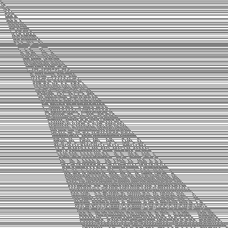
Fixed points are determined directly by running the Global Controlled CA. The Algorithm detects, if a cell belongs to foreground or background. If no cell belongs to the foreground, the fixed point is reached and the algorithm stops.
Example for a Global Controlled CA whose evaluation stops
In[]:=
Image[1-RectangularGCCA[GCCA[{26,235},{{1},0},750]],ImageSize750]
Out[]=

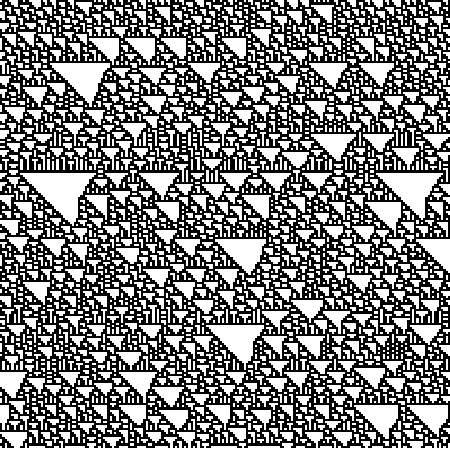
Other Global Controlled CA with more or less complex behavior run the given number of steps:
In[]:=
Show[ImageTake[Image[1-RectangularGCCA[GCCA[{11,28},{{1},0},750]]],All,{750,-1}],ImageSize750]
Out[]=

Detection of periodic patterns
Detection of periodic patterns
Periodic patterns can be detected using the function . In the case of unlimited width the function should be limited to diagonals or columns.
FindTransientRepeat
This codes extract a left diagonal, a right diagonal and a column respectively and find periodic patterns.
In[]:=
LeftDiagonalPeriodicyCheck[tca_,column_]:=LeftDiagonalPeriodicyCheck[tca,column,2];LeftDiagonalPeriodicyCheck[tca_,column_,repeats_]:=FindTransientRepeat[Join[tca[[1;;Floor[column/2],2]],tca[[(1+Floor[column/2]);;-1,1,column]]],repeats];RightDiagonalPeriodicyCheck[tca_,column_]:=RightDiagonalPeriodicyCheck[tca,column,2];RightDiagonalPeriodicyCheck[tca_,column_,repeats_]:=FindTransientRepeat[Join[tca[[1;;Floor[column/2],2]],tca[[(1+Floor[column/2]);;-1,1,-column]]],repeats];ColumnPeriodicyCheck[tca_,column_]:=ColumnPeriodicyCheck[tca,column,2];ColumnPeriodicyCheck[tca_,column_,repeats_]:=FindTransientRepeat[Join[tca[[1;;Abs[column],2]],Extract[tca[[1+Abs[column];;Length[tca],1]],Array[{#,If[column>0,2column+#,#]}&,Length[tca]-Abs[column]]]],repeats];
Periodic patterns can occur, even in very complex patterns such as ECA rule 30. The column index or diagonal can be adjusted using the sliders. Diagonals are parametrized from the left or right. The first column in the manipulate shows the transient before the periodic part (due to its lengths it is displayed as a matrix but it corresponds to a single long list), the second list is the actual periodic part.
In[]:=
testdata=GCCA[{30,30},{{1},0},1500];Manipulate[Panel[Grid[{{"","transient pattern (huge parts are displayed as matrices, zero-length outputs are omitted)","repeated pattern"},Flatten@{"left diagonal:",{If[Length[#[[1]]]==0,"",MatrixForm@Partition[PadRight[#[[1]],Ceiling[Length[#[[1]]],50],""],50]],MatrixForm@{#[[2]]}}&[LeftDiagonalPeriodicyCheck[testdata,l]]},Flatten@{"column:",{If[Length[#[[1]]]==0,"",MatrixForm@Partition[PadRight[#[[1]],Ceiling[Length[#[[1]]],50],""],50]],MatrixForm@{#[[2]]}}&[ColumnPeriodicyCheck[testdata,col]]},Flatten@{"right diagonal:",{If[Length[#[[1]]]==0,"",MatrixForm@Partition[PadRight[#[[1]],Ceiling[Length[#[[1]]],50],""],50]],MatrixForm@{#[[2]]}}&[RightDiagonalPeriodicyCheck[testdata,r]]}},Alignment{{Right,Center,Center}}]],{l,1,10,1},{col,-20,20,1},{r,1,10,1}]
Out[]=

This analyses the same cellular automaton but shows only the lengths of the patterns:
In[]:=
Manipulate[Panel[Grid[{{"","transient pattern length","repeated pattern length"},Flatten@{"left diagonal:",Map[Length,LeftDiagonalPeriodicyCheck[testdata,l],{1}]},Flatten@{"column:",Map[Length,ColumnPeriodicyCheck[testdata,col],{1}]},Flatten@{"right diagonal:",Map[Length,RightDiagonalPeriodicyCheck[testdata,r],{1}]}},Alignment{{Right,Center,Center}}]],{l,1,10,1},{col,-20,20,1},{r,1,10,1}]
Out[]=

Cellular Automata with an overall periodic pattern show repeated patterns in every measured direction at (almost) all columns and diagonals:
In[]:=
testdata2=GCCA[{11,28},{{1},0},750];Manipulate[Panel[Grid[{{"","transient pattern length","repeated pattern length"},Flatten@{"left diagonal:",Map[Length,LeftDiagonalPeriodicyCheck[testdata2,l],{1}]},Flatten@{"column:",Map[Length,ColumnPeriodicyCheck[testdata2,col],{1}]},Flatten@{"right diagonal:",Map[Length,RightDiagonalPeriodicyCheck[testdata2,r],{1}]}},Alignment{{Right,Center,Center}}]],{l,1,10,1},{col,-20,20,1},{r,1,10,1}]
Out[]=

Nevertheless, there are left diagonals and columns, where that cannot be properly detected. The reason is that these diagonals and columns hit the remaining structure after step 558.
Detection of nested patterns
Detection of nested patterns
Under certain circumstances, nested patterns can also be detected using the measures above. In all directions there are either periodic patterns or simply constant values. The detected periods double at an exponential decreasing rate; often this behaviour is detected in two or even three directions. Nevertheless, in deformed nested patterns this does not work, it is even possible that patterns seem chaotic if an unfavorable direction is analysed.
In[]:=
testdata3=GCCA[{90,18},{{1},0},750];Manipulate[Panel[Grid[{{"","transient pattern length","repeated pattern length"},Flatten@{"left diagonal:",Map[Length,LeftDiagonalPeriodicyCheck[testdata3,l],{1}]},Flatten@{"column:",Map[Length,ColumnPeriodicyCheck[testdata3,col],{1}]},Flatten@{"right diagonal:",Map[Length,RightDiagonalPeriodicyCheck[testdata3,r],{1}]}},Alignment{{Right,Center,Center}}]],{l,1,50,1},{col,-50,50,1},{r,1,50,1}]
Out[]=

Detection of chaotic patterns
Detection of chaotic patterns
Although even in very complex rules like rule 30 periodic behaviour can be observed (as actually done in the first example), chaotic patterns can rarely be characterized by the periodic tests we used above. In order to get an idea, what’s going on, we used statistical measures like entropy, mean and standard deviation. These methods are widely used in the following section.
Methods based on pattern-matching will be part of future research.
Parameter space analysis for different coupling parameters
Parameter space analysis for different coupling parameters
Statistics on one global controlled cellular automaton with random initial conditions
Statistics on one global controlled cellular automaton with random initial conditions
In this section CA will be investigated where the next rule is determined by the fraction of black cells. The threshold-fraction is variable here and the Rules for the cellular automaton are fixed. First, a single global controlled CA with random initial conditions is investigated.
In[]:=
SeedRandom[1234];seed1=RandomInteger[{0,1},70];plotdata1=Table[{a,RectangularGCCA[GCCAMajority[{3,18},{seed1,0},a,30]][[All,36;;-37]]},{a,0.,1.,1/99.}];
In[]:=
Map[Image[1-#[[2]],ImageSize300]&,plotdata1]
Tooltips are pre-calculated for the plot:
In[]:=
tooltips1=Map[Column@{Style[FindDistribution[Flatten@plotdata1[[#,2]]],"Subsubsection"],Image[1-plotdata1[[#,2]],ImageSize->240]}&,Range[100]];
In[]:=
Panel[Column@{Column[{Style["entropy","Subsubsection"],ListLinePlot[Table[Tooltip[{plotdata1[[i,1]],N@Entropy[Flatten@plotdata1[[i,2]]]},tooltips1[[i]]],{i,100}],ImageSize{300,220}]},Center],Column[{Style["mean","Subsubsection"],ListLinePlot[Table[Tooltip[{plotdata1[[i,1]],N@Mean[Flatten@plotdata1[[i,2]]]},tooltips1[[i]]],{i,100}],ImageSize{300,223}]},Center],Column[{Style["standard deviation","Subsubsection"],ListLinePlot[Table[Tooltip[{plotdata1[[i,1]],N@StandardDeviation[Flatten@plotdata1[[i,2]]]},tooltips1[[i]]],{i,100}],ImageSize{300,220}]},Center]}]
Out[]=
| ||
| ||
|
Statistics on several global controlled cellular automata
Statistics on several global controlled cellular automata
Mean over 5 cellular automata with different random initial conditions:
In[]:=
SeedRandom[1234];seed2=RandomInteger[{0,1},{5,70}];data2=Table[Table[{a,RectangularGCCA[GCCAMajority[{3,18},{seed2[[part]],0},a,30]][[All,36;;-37]]},{a,0.,1.,1/99.}],{part,5}];
In[]:=
Map[Image[1-#,ImageSize300]&,Map[Mean,Transpose@data2[[All,All,2]],{1}]]
In[]:=
plotdata2=MapIndexed,#&,Map[Mean,Transpose@data2[[All,All,2]],{1}];
#2[[1]]-1
99
Tooltips are pre-calculated for the plot :
In[]:=
tooltips2=Map[Column@{Style[FindDistribution[Flatten@plotdata2[[#,2]]],"Subsubsection"],Image[1-plotdata2[[#,2]],ImageSize->240]}&,Range[100]];
In[]:=
Panel[Column@{Column[{Style["entropy","Subsubsection"],ListLinePlot[Table[Tooltip[{plotdata2[[i,1]],N@Entropy[Flatten@plotdata2[[i,2]]]},tooltips2[[i]]],{i,100}],ImageSize{300,220}]},Center],Column[{Style["mean","Subsubsection"],ListLinePlot[Table[Tooltip[{plotdata2[[i,1]],N@Mean[Flatten@plotdata2[[i,2]]]},tooltips2[[i]]],{i,100}],ImageSize{300,223}]},Center],Column[{Style["standard deviation","Subsubsection"],ListLinePlot[Table[Tooltip[{plotdata2[[i,1]],N@StandardDeviation[Flatten@plotdata2[[i,2]]]},tooltips2[[i]]],{i,100}],ImageSize{300,220}]},Center]}]
Out[]=
| ||
| ||
|
Mean over 50 cellular automata with different random initial conditions. In this case, it is also shown, how these statistical measures stabilize, if one increases the number of steps.:
In[]:=
SeedRandom[1234];seed3=RandomInteger[{0,1},{50,70}];data3=Table[Table[{a,RectangularGCCA[GCCAMajority[{3,18},{seed3[[part]],0},a,30]][[All,36;;-37]]},{a,0.,1.,1/99.}],{part,50}];
In[]:=
plotdata3=MapIndexed,#&,Map[Mean,Transpose@data3[[All,All,2]],{1}];
#2[[1]]-1
99
Tooltips are pre-calculated for the plot :
In[]:=
tooltips3=Map[Column@{Style[FindDistribution[Flatten@plotdata3[[#,2]]],"Subsubsection"],Image[1-plotdata3[[#,2]],ImageSize->240]}&,Range[100]];
In[]:=
plots3=Map[Panel[Column@{Column[{Style["entropy","Subsubsection"],ListLinePlot[Table[Tooltip[{plotdata3[[i,1]],N@Entropy[Flatten@plotdata3[[i,2,1;;#]]]},tooltips3[[i]]],{i,100}],ImageSize{300,220}]},Center],Column[{Style["mean","Subsubsection"],ListLinePlot[Table[Tooltip[{plotdata3[[i,1]],N@Mean[Flatten@plotdata3[[i,2,1;;#]]]},tooltips3[[i]]],{i,100}],ImageSize{300,223}]},Center],Column[{Style["standard deviation","Subsubsection"],ListLinePlot[Table[Tooltip[{plotdata3[[i,1]],N@StandardDeviation[Flatten@plotdata3[[i,2,1;;#]]]},tooltips3[[i]]],{i,100}],ImageSize{300,220}]},Center]}]&,Range[31]];
In[]:=
Panel[Column@{Column[{Style["entropy","Subsubsection"],ListLinePlot[Table[Tooltip[{plotdata3[[i,1]],N@Entropy[Flatten@plotdata3[[i,2]]]},tooltips3[[i]]],{i,100}],ImageSize{300,220}]},Center],Column[{Style["mean","Subsubsection"],ListLinePlot[Table[Tooltip[{plotdata3[[i,1]],N@Mean[Flatten@plotdata3[[i,2]]]},tooltips3[[i]]],{i,100}],ImageSize{300,223}]},Center],Column[{Style["standard deviation","Subsubsection"],ListLinePlot[Table[Tooltip[{plotdata3[[i,1]],N@StandardDeviation[Flatten@plotdata3[[i,2]]]},tooltips3[[i]]],{i,100}],ImageSize{300,220}]},Center]}]
Out[]=
| ||
| ||
|
Determine the effect of the number of calculated rows on the statistical measures
In[]:=
Manipulate[plots3[[n]],{n,1,31,1}]
Out[]=

Parameter space analysis for different combinations of CAs
Parameter space analysis for different combinations of CAs
This section contain statistics of all possible combinations of CA where the next rule is determined by the fraction of black cells. The threshold-fraction is fixed at 1/2 for this plot. Both plots show the same data but the first one is without interpolation.
In[]:=
SeedRandom[1234];seed256=RandomInteger[{0,1},90];
In[]:=
data256=TableTablei,j,RectangularGCCAGCCAMajority{i,j},{seed256,0},,30[[All,36;;-37]],{i,0,255},{j,0,255};
1
2
ListPlot3D[Flatten[Table[{data256[[i+1,j+1,1]],data256[[i+1,j+1,2]],N@Mean[Flatten@data256[[i+1,j+1,3]]]},{i,0,255},{j,0,255}],1],BoxRatios1,PlotRangeFull,(*AxesOrigin->{0,0,0},*)ImageSize700,AxesStyleDirective[20],AxesLabelMap[Style[#,Bold,28]&,{"rule i","rule j","mean"}],InterpolationOrder0]
Out[]=

In[]:=
ListPlot3D[Flatten[Table[{data256[[i+1,j+1,1]],data256[[i+1,j+1,2]],N@Mean[Flatten@data256[[i+1,j+1,3]]]},{i,0,255},{j,0,255}],1],BoxRatios1,PlotRangeFull,(*AxesOrigin->{0,0,0},*)ImageSize700,AxesStyleDirective[20],AxesLabelMap[Style[#,Bold,28]&,{"rule i","rule j","mean"}]]
Out[]=

Behavior of globally coupled CAs for different coupling functions
Behavior of globally coupled CAs for different coupling functions
These systems are very sensitive to changes in boths, initial conditions and the size of the system.
For example, the system whose applied rule depends on whether the number of black cells is even or odd would behave differently, when odd rule numbers are involved. More precisely, there are three cases to distinguish:
1) the system is infinite and/or only the cells of the foreground are counted.
2) the system is finite and has an even width, all cells are counted.
3) the system is finite and has an odd width, all cells are counted.
Rules with an odd rule number have the property that black lines across the whole CA can appear whenever that rule is applied. Therefore, if at least one of the rules we combine has an odd rule number, it has an effect if the background cells are counted or not and if the width of the CA is even or odd. Depending on the case the behaviour of the system can be completely different:
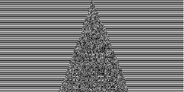
As an example we look at the system rule 11 (class 2) and rule 28 (class 2). The result of the first case begins like a class 3 system but ends with class 2 behaviour.
For example, the system whose applied rule depends on whether the number of black cells is even or odd would behave differently, when odd rule numbers are involved. More precisely, there are three cases to distinguish:
1) the system is infinite and/or only the cells of the foreground are counted.
2) the system is finite and has an even width, all cells are counted.
3) the system is finite and has an odd width, all cells are counted.
Rules with an odd rule number have the property that black lines across the whole CA can appear whenever that rule is applied. Therefore, if at least one of the rules we combine has an odd rule number, it has an effect if the background cells are counted or not and if the width of the CA is even or odd. Depending on the case the behaviour of the system can be completely different:
As an example we look at the system rule 11 (class 2) and rule 28 (class 2). The result of the first case begins like a class 3 system but ends with class 2 behaviour.
In[]:=
ImageTake[Image[1-RectangularGCCA[GCCA[{11,28},{{1},0},750]]],All,{751,-1}]
Out[]=

In[]:=
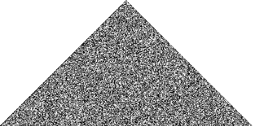
Image[1-GCCAWithBackground[{11,28},Join[{1},ConstantArray[0,750]],750]]
Out[]=
In[]:=
Image[1-GCCAWithBackground[{11,28},Join[{1},ConstantArray[0,751]],750]]
Out[]=

One can easily see, that these systems are completely different:
in case 1, the system becomes periodic after 558 steps, the evaluation of cases 2 and 3 remains chaotic for a much longer evaluation (it is not known, if they ever become periodic). Note also the obviously different behavior at the left hand side in cases 2 and 3.
in case 1, the system becomes periodic after 558 steps, the evaluation of cases 2 and 3 remains chaotic for a much longer evaluation (it is not known, if they ever become periodic). Note also the obviously different behavior at the left hand side in cases 2 and 3.
Needless to say that differences will also occur (for the same reasons), when the rule depends on the fraction of black cells. But in this case, there are not only three cases but infinitely many - and it occurs for every pair of rule numbers. But this cannot be discussed in detail here.
Emerging Complexity
Emerging Complexity
Effects of Changing a Single Bit in the Initial Condition
Effects of Changing a Single Bit in the Initial Condition
Due to immediate change of the applied rule the change of a single bit in the initial condition will change the global behavior. In opposite to elementary CA, where a changed bit has only local effect which propagate more or less (depending on the rule), there is a huge effect on the whole automaton, if the involved rules are not too simple.
Here are some examples of different behaviour and complexity:
rule 11 and rule 28:
random initial condition:
Out[]=

same random initial condition, one bit changed:
Out[]=

Image difference of the first two images:
Out[]=

The same for rule combination 110-124
Out[]=
Out[]=

Out[]=

Simple Mirrored Rules Yield Complex Behaviour
Simple Mirrored Rules Yield Complex Behaviour
We consider a special group of rules, those where one rule of the CA is exactly the “mirrored” rule of the second one. One could suspect that the CA generated this way behave only very regularly because they basically use “only themselves” and nothing new is generated. However, a systematic search of the 128 (ignoring symmetry) possible combinations shows very interesting examples such as the following:
rule 9 (class 2) and rule 65 (class 2), result: (class 2)

rule 61 (class 2) and rule 103 (class 2), result: (class 4 or class 3, difficult to determine)
rule 62 (class 2) and rule 118 (class 2), result: (class 4 or class 2, difficult to determine)

rule 30 (class 3) and rule 86 (class 3): result: (class 3)
rule 110 (class 4) and rule 124 (class 4): result: (class 3)
The following code can be used to perform the search for mirrored rules.
In[]:=
Manipulate[Column@Map[RulePlot[CellularAutomaton[#]]&,{n,FromDigits[Extract[IntegerDigits[n,2,8],Transpose@{{1,5,3,7,2,6,4,8}}],2]}],{n,0,255,1}]
Out[]=
|  | ||||||||
|

Concluding remarks
Concluding remarks
We have observed some very interesting properties of globally controlled CA which usual CA do not share, for example the strong dependence on the parity of rules and automaton width. These imply that the additional structure which we added through combining the rules based on some criterion strongly increases the system’s sensitivity to initial conditions and the variety of possible systems, however only when the rule decision parameters of the GCCA are in a certain range (outside that range, the statistical values stabilize as above).
Especially interesting is the observation that this effect exists even if the systems of which a GCCA is composed are not very sensitive to initial conditions, meaning that the way in which we combined the rules yields emergent behaviour regarding the sensitivity of CA to initial conditions. Also, we have found examples of class 2 which, when combined, give class 3 or 4 CA and also examples where GCCA composed of class 4 automata show class 3 behaviour.
Especially interesting is the observation that this effect exists even if the systems of which a GCCA is composed are not very sensitive to initial conditions, meaning that the way in which we combined the rules yields emergent behaviour regarding the sensitivity of CA to initial conditions. Also, we have found examples of class 2 which, when combined, give class 3 or 4 CA and also examples where GCCA composed of class 4 automata show class 3 behaviour.
Keywords
Keywords
◼
Cellular Automaton
◼
Global Control
◼
A New Kind of Scince
Acknowledgment
Acknowledgment
I want to thank Stephen Wolfram for defining this project for me. I also want to thank my mentor Marco Thiel for many helpful discussions. Furthermore, I want to thank Jesse Friedman, Silvia Hao, Carlos Muñoz, Daniel Sanchez, Nikolay Murzin and Samuele Mongodi for help on my project related chat questions. Finally, I want to thank Yorick Zeschke for his really important help at the last day before project submission.
References
References
◼
Stephen Wolfran (2002), A new kind of science, Wolfram Media
Cite this as: Andreas Mämpel, "[WSS 2021] Cellular Automata with Global Control" from the Notebook Archive (2021), https://notebookarchive.org/2021-07-62hwu8u
Download
