Modeling the Center of Mass for College Mechanics
Author
Stephan Bourget
Title
Modeling the Center of Mass for College Mechanics
Description
Teacher notebook for an WL-based approach to center of mass.
Category
Essays, Posts & Presentations
Keywords
center of mass, mass distribution, mechanics, college physics, physics education
URL
http://www.notebookarchive.org/2021-07-6fliiur/
DOI
https://notebookarchive.org/2021-07-6fliiur
Date Added
2021-07-14
Date Last Modified
2021-07-14
File Size
279.59 kilobytes
Supplements
Rights
CC BY 4.0

WOLFRAM SUMMER SCHOOL 2021
Modeling the Center of Mass for College Mechanics
Modeling the Center of Mass for College Mechanics
Stephan Bourget, M.Ed.
Vanier College, Montreal, Quebec, Canada
College introductory physics students experience a lot of conflicting misconceptions when they study Newtonian mechanics, which modeling instruction helps to address. The difficulty nevertheless compounds in the study of rotational kinematics and dynamics, with the addition of a new notation with vector products and vectors normal to the plane of rotation. It is here proposed to use the power of computational modeling through the Wolfram Language to facilitate the visualization and solving of rotational problems, in the hope that it brings a greater grasp of the concepts and a greater ability to go through the mathematics and focus on the physics. Furthermore, computational modeling is now an indispensable skill and component of scientific work, which complements the other two traditional components: experimenting and theorizing. Therefore, this project presents the first section of the first edition of a Wolfram Language notebook to teach rotational kinematics and dynamics interactively while allowing students to play with demonstrations and use simple code to solve problems, bringing their attention to the conceptual setup rather than on the mathematical details that they they’ll learn in their concomitant Calculus I course, and in their future Calculus II and Linear Algebra courses. The next step is to test this notebook in class and see how it impacts student learning. If results seem positive, then further units of Mechanics first, and other courses later, should be converted, and the use of the Wolfram Language as a basis for instruction could be broaden. This is particularly important in the context of a Science program revision in Quebec’s CEGEP system, which enlarge the role of computer skills in the educational training of students.
Project Outcomes
Project Outcomes
◼
Development of teacher notebook for the first section of the unit on rotational kinematics and dynamics, namely the section on the center of mass.
◼
Integration of useful Wolfram demonstrations.
◼
Integration of Wolfram computation to solve some pertinent problems based on a careful symbolic conceptual setup, leaving the intricacies of the mathematics to the computer.
◼
As an aside, a simulation of projectile motion with drag and a second-law-of-Newton solver featuring a force diagram were produced while learning to code. Those computational artefacts will be useful in other units of the mechanics course, the latter being also useful as a bridge to analyze static equilibrium in rotation.
Refresher
Refresher
Basic types of motion
Basic types of motion
At the start of the course, we defined 3 basic types of motion (and the idea that more complicated motion can be understood as a combination of the basic types):
◼
Translation: Object moves through space from point A to B (while keeping its orientation).
◼
Rotation: Object rotates about some axis.
◼
Oscillation: Object oscillates about some equilibrium point.
"Point-like" particles
"Point-like" particles
So far, we have assumed that all objects could be considered as “point-like particles”:
◼
They have a position... but occupy no space!
◼
They can move with velocity and acceleration.
◼
They have mass.
◼
Forces can be applied to them by agents.
These assumptions are fairly valid for the translational motion of inflexible objects, but if the “point-like objects” we’re considering do not have the property of size, then the concept of rotating around their axis does not exist.
Therefore, if we want to consider the rotational properties of objects, we will need to consider the size and shape of the object, and how its mass is distributed throughout its size and shape.
Therefore, if we want to consider the rotational properties of objects, we will need to consider the size and shape of the object, and how its mass is distributed throughout its size and shape.
Mass distribution
Mass distribution
The simplest type of mass distribution is a single point-like particle with all its mass located at a single point (of negligible size).
We could also have a mass distribution made of several discrete point-like particles of mass each located at different points in space.
A “real” (or “extended”) object can be modelled as a continuous distribution of an arbitrarily large (or infinite) number of point-like particles spread throughout the volume of the object.
We could also have a mass distribution made of several discrete point-like particles of mass
{,,,…}
m
1
m
2
m
3
A “real” (or “extended”) object can be modelled as a continuous distribution of an arbitrarily large (or infinite) number of point-like particles spread throughout the volume of the object.
Center of mass (CM or CoM)
Center of mass (CM or CoM)
The center of mass of a system of particles is the point that moves as though…
◼
All of the system’s mass were concentrated there.
◼
All external forces were applied there.
In[]:=
Hyperlink["MIT Physics Demo -- Center of Mass Trajectory","https://www.youtube.com/watch?v=DY3LYQv22qY"]
For the case of either a discrete or continuous mass distribution, the “center of mass” is like an average position for the distribution of mass through space (either 1D, 2D or 3D).
◼
The center of mass (CM) is averaged over the entire mass distribution.
◼
It may not necessarily be located (physically) within the object.
◼
If an object (or mass distribution) is allowed to rotate freely, it will naturally rotate about an axis that passes through the center of mass.
◼
The center of mass can be considered as a "balance point" within an object.
Distribution of 2 point-like particles
Distribution of 2 point-like particles
A system of two point-like particles of mass defines a 1-dimensional line between the two points.
{,}
m
1
m
2
The center of mass position (defined with respect to the chosen origin) will lie somewhere on this line, between the two masses.
x
CM
Notice: is closer to the larger of the two masses.
x
CM
x
CM
m
1
x
1
m
2
x
2
m
1
m
2
In[]:=
Manipulate[ |
Out[]=
|  | ||||||||||||||||||||||||||||||||||
|


Distribution of 3 point-like particles
Distribution of 3 point-like particles
Any three point-like particles of mass can form a 2D plane, and the center of mass for this distribution will lie somewhere within this 2D plane, with coordinates .
{,,}
m
1
m
2
m
3
(,)
x
CM
y
CM
x
CM
m
1
x
1
m
2
x
2
m
3
x
3
m
1
m
2
m
3
and
y
CM
m
1
y
1
m
2
y
2
m
3
y
3
m
1
m
2
m
3
that is
r
CM
m
1
r
1
m
2
r
2
m
3
r
3
m
1
m
2
m
3
In[]:=
Manipulate[ |
Out[]=
| | ||||||||||||||||||||||||||||||||||||||||||||||||
| |||||||||||||||||||||||||||||||||||||||||||||||||
Exercise 1
Exercise 1
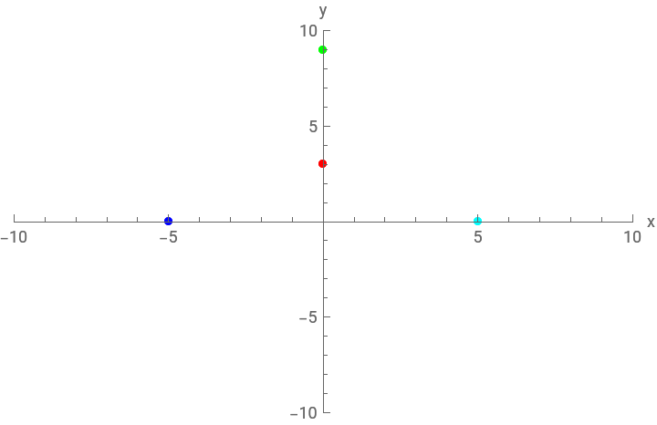
Three particles of masses = {1.20, 2.50, 3.40} kg form an equilateral triangle of edge length = 140 cm. Where is the center of mass of this system?
{,,}
m
1
m
2
m
3
a
[Answer: At 82.8 cm along the edge toward the 2.50-kg particle, 58.1 cm perpendicular to that same edge and inward, from the 1.20-kg particle.]
In[]:=
{m1,m2,m3}={1.20,2.50,3.40};
kg
In[]:=
a=140;h=-;
2
a
2
a
2
In[]:=
{r1,r2,r3}={0,0},{a,0},,h;
a
2
cm
In[]:=
rCM=
m1r1+m2r2+m3r3
m1+m2+m3
Out[]=
,
82.8169
cm
58.0603
cm
In[]:=
ListPlot[ |
Out[]=
 |
|
Distribution of n point-like particles
Distribution of n point-like particles
A distribution of n point-like particles of mass {, , , , …, ,} can potentially occupy a 3D volume, and the center of mass for this distribution will have coordinates (, , ).
m
1
m
2
m
3
m
4
m
n
x
CM
y
CM
z
CM
x
CM
x
1
m
1
x
2
m
2
x
3
m
3
x
4
m
4
x
n
m
n
m
1
m
2
m
3
m
4
m
n
n
∑
i=1
x
i
m
i
M
tot
y
CM
y
1
m
1
y
2
m
2
y
3
m
3
y
4
m
4
y
n
m
n
m
1
m
2
m
3
m
4
m
n
n
∑
i=1
y
i
m
i
M
tot
z
CM
z
1
m
1
z
2
m
2
z
3
m
3
z
4
m
4
z
n
m
n
m
1
m
2
m
3
m
4
m
n
n
∑
i=1
y
i
m
i
M
tot
that is
r
CM
r
1
m
1
r
2
m
2
r
3
m
3
r
4
m
4
r
n
m
n
m
1
m
2
m
3
m
4
m
n
n
∑
i=1
r
i
m
i
M
tot
In[]:=
DynamicModule[ |
Out[]=
Number of particles 3 | |||||||||||||||||||||||||||
| |||||||||||||||||||||||||||
| |||||||||||||||||||||||||||
|

Continuous mass distributions (enrichment)
Continuous mass distributions (enrichment)
An actual physical object can be modelled as a continuous mass distribution, spread throughout its volume. The center of mass still has the same concept as an “average position”. To actually calculate the center of mass for a continuous distribution, we need to add up an infinite amount of infinitesimally small point-masses m, of volume V = x y z (Cartesian coordinate system) = r r θ z (cylindrical coordinate system) = Sin[ϕ] r ϕ θ (spherical coordinate system), then find the integral of this mass distribution (you will learn about integrals formally in Calculus II).
2
r
x
CM
lim
n∞
n
∑
i=1
x
i
m
i
M
tot
M
tot
∫
0
M
tot
V
tot
∫
0
M
tot
∫∫∫xρ(x,y,z)xyz
M
tot
y
CM
lim
n∞
n
∑
i=1
y
i
m
i
M
tot
M
tot
∫
0
M
tot
V
tot
∫
0
M
tot
∫∫∫yρ(x,y,z)xyz
M
tot
z
CM
lim
n∞
n
∑
i=1
y
i
m
i
M
tot
M
tot
∫
0
M
tot
V
tot
∫
0
M
tot
∫∫∫zρ(x,y,z)xyz
M
tot
that is
r
CM
lim
n∞
n
∑
i=1
r
i
m
i
M
tot
M
tot
∫
0
r
M
tot
V
tot
∫
0
r
r
M
tot
In[]:=
Manipulate[ |
Out[]=
| | |||||||||||||||||||||||||||||||||
| ||||||||||||||||||||||||||||||||||

Exercise 1
Exercise 1
A rectangular prism of length l, width w, and height has a density . Its mass is unknown. Where is its center of mass?
zh
ρ=kz
In[]:=
position={x,y,z};
In[]:=
ρ=k*z;
In[]:=
M
tot
h
∫
0
w
∫
0
l
∫
0
In[]:=
positionCM={xCM,yCM,zCM}->(position)ρxyz
h
∫
0
w
∫
0
l
∫
0
M
tot
Out[]=
{xCM,yCM,zCM},,
l
2
w
2
2h
3
Exercise 2
Exercise 2
A cylinder or radius R and height z = h has a density . Its mass is unknown. Where is its center of mass?
ρ=kz
In[]:=
position={x,y,z}={rCos[θ],rSin[θ],z};
In[]:=
ρ=k*z;
In[]:=
M
tot
h
∫
0
2π
∫
0
R
∫
0
In[]:=
positionCM={xCM,yCM,zCM}->(position)ρrrθz
h
∫
0
2π
∫
0
R
∫
0
M
tot
Out[]=
{xCM,yCM,zCM}0,0,
2h
3
Exercise 3
Exercise 3
A sphere or radius R has a density . Its mass is unknown. Where is its center of mass?
ρk(R+z)k(R+rcos(ϕ))
In[]:=
position={x,y,z}={rSin[ϕ]Cos[θ],rSin[ϕ]Sin[θ],rCos[ϕ]};
In[]:=
ρ=k(R+z);
In[]:=
M
tot
2π
∫
0
π
∫
0
R
∫
0
2
r
In[]:=
positionCM={xCM,yCM,zCM}->(position)ρSin[ϕ]rϕθ
2π
∫
0
π
∫
0
R
∫
0
2
r
M
tot
Out[]=
{xCM,yCM,zCM}0,0,
R
5
Extra demonstrations
Extra demonstrations
Center of mass in a canoe
Center of mass in a canoe
In[]:=
ResourceData["Demonstrations Project: Center of Mass in a Canoe"]
Out[]=
| | ||||||||||||||||||||||||
| |||||||||||||||||||||||||

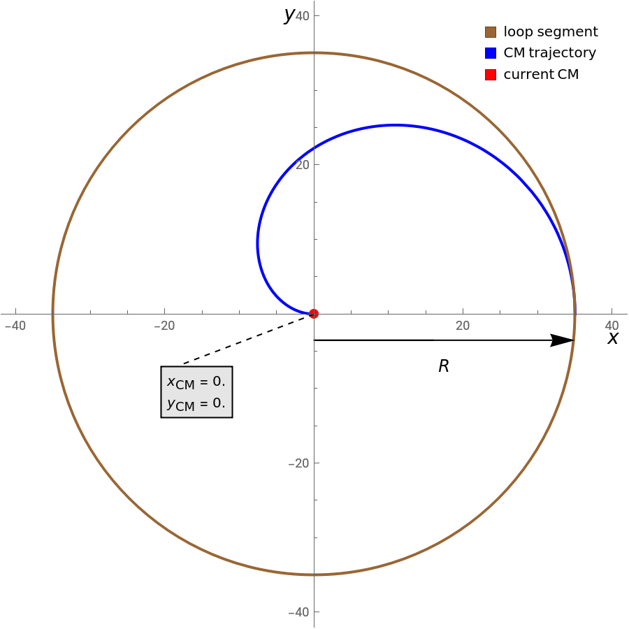
Center of mass of a circular arc
Center of mass of a circular arc
In[]:=
ResourceData["Demonstrations Project: Center of Mass of a Circular Arc"]
Out[]=
| | ||||||||||||
| |||||||||||||
Center of mass of a perforated square plate
Center of mass of a perforated square plate
In[]:=
ResourceData["Demonstrations Project: Center of Mass of a Perforated Square Plate"]
Out[]=
| | ||||||||||||||||||||||||
| |||||||||||||||||||||||||

Center of mass of a polygon
Center of mass of a polygon
Use -click on Windows, -click on Mac, or -click on Linux to create additional vertices.
In[]:=
ResourceData["Demonstrations Project: Center of Mass of a Polygon"]
Out[]=
| | |||||||||
| ||||||||||

Empirical method for finding the center of mass for an irregularly shaped object
Empirical method for finding the center of mass for an irregularly shaped object
◼
We should understand that even for complicated objects, the center of mass will tend to be closer to the more massive parts (i.e., a hammer head), but can also be “pulled away” by a smaller mass that is spread further away (like a dinosaur tail).
◼
The line of the gravitational force always acts through the center of mass.
◼
In many cases, we'll simply be told where the center of mass is located.
◼
For objects with a uniform mass distribution (or uniform mass density), the center of mass is located at the geometrical center of the object.
What about our previous point-like particle approximation?
What about our previous point-like particle approximation?
If we are studying the translational properties of an object that does not flex or deform or change it’s shape... we can simply study the behaviour of the center of mass (and the rest of the object follows the physics of its center of mass).
◼
Kinematics:
,,,…
r
CM
v
CM
a
CM
◼
Dynamics:
m,…
F
CM
a
CM
◼
Energy:
,mg,…
E
k,trans
m
2
v
CM
2
E
g
h
CM
◼
Momentum:
=m,…
p
CM
v
CM
◼
Etc.
Exercise 1
Exercise 1
A 60.0-kg person is at the left end of a 5.00-m long canoe having a mass of 90.0 kg. She then moves to the right end of the canoe. In both cases, she is 60.0 cm from the end of the canoe. By how much has the canoe shifted if there is no friction between the canoe and the water?
[Answer: Shift of 1.52 m toward the left.]
In[]:=
{massPerson,massCanoe}={60.0,90.0};lengthCanoe=5.00;initialPositionCanoe=0;initialPositionPerson=initialPositionCanoe-lengthCanoe/2+0.600;finalPositionCanoe=initialPositionCanoe+shift;finalPositionPerson=finalPositionCanoe+lengthCanoe/2-0.600;initialCM=;finalCM=;soln=SolveValues[initialCM==finalCM,shift];shiftValue=soln[[1]];"Shift: "<>ToString[shiftValue]
kg
m
m
m
m
(massPerson)(initialPositionPerson)+(massCanoe)(initialPositionCanoe)
massPerson+massCanoe
(massPerson)(finalPositionPerson)+(massCanoe)(finalPositionCanoe)
massPerson+massCanoe
Out[]=
Shift: -1.52 meters
In[]:=
finalPositionCanoe=initialPositionCanoe+shiftValue;finalPositionPerson=finalPositionCanoe+lengthCanoe/2-0.600;finalCM=;
m
massPersonfinalPositionPerson+massCanoefinalPositionCanoe
massPerson+massCanoe
NumberLinePlot[ |
Out[]=
 |
|
Concluding remarks
Concluding remarks
This work was only a first step toward a complete revision of teaching notes for rotation in a college introductory mechanics course. The plan is to complete the set of notes, develop a student workbook to foster further engagement with the Wolfram Language, and test their use in an actual classroom, looking for positive effect on learning outcomes, before expanding the use of notebooks to all units of the course.
Appendix 1: Air Drag Effect on Projectile Motion
Appendix 1: Air Drag Effect on Projectile Motion
On my way to learn the Wolfram Language, I found an article by de Alwis (2000), in which code based on Mathematica 3.0 and run on Windows 95 was provided to compare projectile motion with and without air drag. An attempt was made to adapt the code to Mathematica 12.3, which would be useful when studying projectile motion in mechanics.
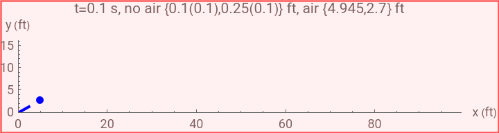
Projectiles with and without air resistance.
In[]:=
v=60(*ft/s*);theta=20Degree(*°*);m=2(*kg*);b=3;g=32(*ft/s^2*);r=v^2*Sin[2*theta]/g;h=v^2*(Sin[theta])^2/(2*g);T=v*Sin[theta]/g;Tair=m*Log[1+b*v*Sin[theta]/(m*g)]/b;x[t_]:=v*Cos[theta]*t;y[t_]:=v*Sin[theta]*t-g*t^2/2;xair[t_]:=m*v*Cos[theta](1-Exp[-b*t/m])/b;yair[t_]:=(m^2*g/b^2+m*v*Sin[theta]/b)*(1-Exp[-b*t/m])-m*g*t/b;
s=FindRoot[yair[t]==0,{t,2*T}];Print["h=",N[h]];Print["r=",N[r]];Print["h[air]=",N[yair[t]/.t->Tair]];Print["r[air]=",N[xair[t]/.s]]
Manipulate[ |
Out[]=
| | ||||||
| |||||||
h=6.58
r=72.3136
h[air]=4.09603
r[air]=29.5481
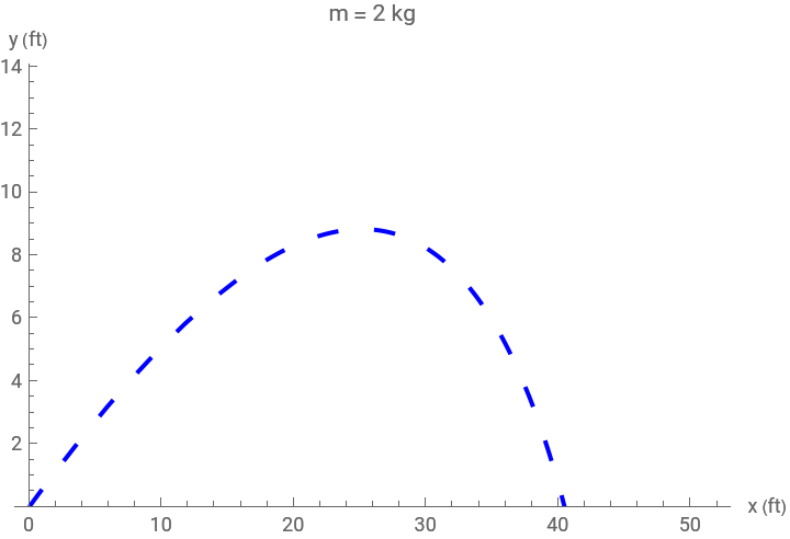
Effect of mass on the air resistance.
In[]:=
v=60(*ft/s*);theta=30Degree;g=32(*ft/s^2*);mmin=10(*kg*);mmax=310(*kg*);d=25;b=2;h=v^2*(Sin[theta])^2/(2*g);r=v^2*Sin[2*theta]/g;y[x_]:=x*Tan[theta]-g*x^2/(2*v^2*Cos[theta]^2)
Manipulate[ |
Out[]=
| | ||||||
| |||||||
Keywords
Keywords
◼
center of mass
◼
mass distribution
◼
mechanics
◼
college physics
◼
physics education
Acknowledgment
Acknowledgment
I would like to thank the generous help offered by my mentors Paul Abbott and Santiago Camacho, along with teaching assistants Jesse Friedman, Silvia Hao, Daniel Sanchez, and Faizon Zaman. Also many thanks to Stephen Wolfram for setting up the summer school and providing great overall inspiration through his life work, and also for developing the Wolfram Language upon which this project and many others rest.
References
References
◼
Caviness, K. E. (2010). "Center of Mass of a Polygon" in Wolfram Demonstrations Project. Web: http://demonstrations.wolfram.com/CenterOfMassOfAPolygon/
◼
de Alwis, T. (2000). Projectile motion with Mathematica. International Journal of Mathematical Education in Science and Technology, 31(5), 749–55.
◼
Kadonaga, N. (2015). “Center of Mass in a Canoe” in Wolfram Demonstrations Project. Web: http://demonstrations.wolfram.com/CenterOfMassInACanoe/
◼
Mahieu, E. (2015). “Center of Mass of a Perforated Square Plate” in Wolfram Demonstrations Project. Web: http://demonstrations.wolfram.com/CenterOfMassOfAPerforatedSquarePlate/
◼
Silvestre, W. (2019). “Center of Mass of a Circular Arc” in Wolfram Demonstrations Project. Web: http://demonstrations.wolfram.com/CenterOfMassOfACircularArc/
Clear["Global`*"]
Cite this as: Stephan Bourget, "Modeling the Center of Mass for College Mechanics" from the Notebook Archive (2021), https://notebookarchive.org/2021-07-6fliiur
Download
