Visualizing Context in the Meaning Space
Author
Angelo Barona Balda
Title
Visualizing Context in the Meaning Space
Description
This project presents 2D and 3D representations of the meaning space structure. These representations are based in contextual word vectors provided by the ELMo neural network.
Category
Student Work
Keywords
Language Modelling
URL
http://www.notebookarchive.org/2021-07-6hpy57e/
DOI
https://notebookarchive.org/2021-07-6hpy57e
Date Added
2021-07-14
Date Last Modified
2021-07-14
File Size
1.96 megabytes
Supplements
Rights
CC BY 4.0

Visualizing Context in the Meaning Space Structure
Visualizing Context in the Meaning Space Structure
This project presents 2D and 3D representations of the meaning space structure. These representations are based in contextual word vectors provided by the ELMo neural network.
Introduction
Introduction
The meaning space of a language encases all the possible meanings of every object or concept that the language describes. The structure of a meaning space, according to Kirby (2007), consists of an F-number of dimensions. Each dimension corresponds to a feature used in the meaning space to distinguish objects. These features take a specific value V from a set of possible values. In this way, every possible meaning in the space corresponds to an exclusive combination of an F-number of V-values.To create an approximation of the meaning space of English, I used the word vector representation. A word vector is the numerical encoding of the meaning of a word. These word vectors are usually produced by neural networks, which undergo substantial training to identify patterns and relations in a lexicon. The Wolfram Language provides several types of text-related neural networks. For this project, I chose to work with the ELMo network. ELMo produces two contextual and one non-contextual versions of vectors for every word. Each vector contains 1024 elements. This means that the ELMo network interprets the meaning space as a structure of 1024 dimensions.Each dimension can take a value within a range that approximates to a Gaussian distribution with mean = 0 and variance = 0.2. To back this statement, computed the vectors of three random words and plotted a histogram of their values.  Figure 1. Histogram of the Word Vectors of Random WordsIn this project I use the contextual and non-contextual word vectors to provide an approximate visualization of the meaning space structure in the English language. Additionally, I study the role of context in ELMo’s interpretation of meaning and how this interpretation evolves as during text analysis.
Non-Contextual Meaning Space
Non-Contextual Meaning Space
Before analyzing the effects of context, I created a visualization of the non-contextual meaning space as a starting point. This is to provide a general idea of the meaning space structure. For this, I used the non-contextual word vectors provided by ELMo.
As explained in the previous section, ELMo works with a meaning space of 1024, which is difficult to study. To simplify the problem, I applied Principal Components Analysis (PCA) to reduce the dimensionality of the structure to three.
I encased this process, together with the plotting process, in the nonContextSpace function. This function creates a set of random words and computes their three-dimensional word vectors. Then it plots the vectors in a 3D space. To see the implementation details, see the nonContextSpace subsection.
The output of the function is the following:
In[]:=
nonContextSpace
Out[]=
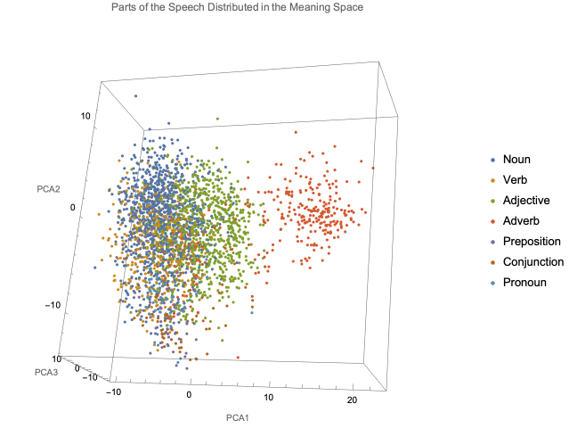
Figure 2. Parts of the Speech Distributed in the Meaning Space
For this experiment, I worked with a set of 2820 random words selected with built-in Wolfram functions. To identify the words more easily, I classified the words by parts of the speech.
Figure 2 shows how most of the parts of the speech are located in close proximity. However, they are clustered in specific regions. The most prominent clusters are those of Nouns, Verbs, Adjectives, and Adverbs. This is because these are the most abundant types of words from those available in the Wolfram Language functions.
In the figure, nouns and verbs are very close to each other, even sharing a significant portion of space. Adjectives are close to nouns and verbs, but have a delimited region. Adverbs are located in their own region separated from the rest of the words.
nonContextSpace
nonContextSpace
Influence of Context in Meaning Identification
Influence of Context in Meaning Identification
For this experiment I worked with the two contextual word vectors provided by the ELMo network. I used these vectors to visualize different definitions of a single word in the meaning space. To simplify the analysis, instead of using random words, I selected four specific words: “rest”, “play”, “head”, and “close”.
WIth each word, I performed the following procedure:
WIth each word, I performed the following procedure:
1
.Create a dataset of 1000 to 4000 Wikipedia sentences that contain the word that I was working with. For this, I created the GetWikiWordText function.
2
.Compute the vectors of the words in each sentence. For this, I created the ComputeWordVectors function.
3
.Plot the word vectors in 2D and 3D spaces. For this, I created the PlotWordData function
To see the implementation details of the functions specified above, see the corresponding subsections at the end of this section.
In the following subsections I describe the results obtained for each of the studied words.
In the following subsections I describe the results obtained for each of the studied words.
Word “Rest”
Word “Rest”
The results for “rest” are the following:
step1=GetWikiWordText["rest",1000];step2=ComputeWordVectors[step1];step3=PlotWordData[step2,2,"Rest"]
Out[]=
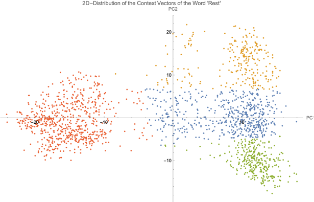
Figure 3. 2D Distribution of the Context Vectors of “Rest”
Each point in Figure 3 represents an instance of the word “rest” in a Wikipedia sentence. The figure shows that the points form four clusters. However, there is a pronounced separation between the red and the other three clusters. The clusters correspond to the following contexts:
Each point in Figure 3 represents an instance of the word “rest” in a Wikipedia sentence. The figure shows that the points form four clusters. However, there is a pronounced separation between the red and the other three clusters. The clusters correspond to the following contexts:
◼
Red Cluster: Sentences where “rest” means the remainder of something.
◼
Orange, Blue, and Green Clusters: Sentences where “rest” means to be in repose or motionless. These three clusters, although they share the same meaning, are divided by context as follows:
◼
Orange Cluster: Sentences related to sleep and relaxation.
◼
Blue Cluster: Sentences related to motionlessness, specially in physics or chemistry.
◼
Green Cluster: Sentences related with religious ceremonies and death.
step1=GetWikiWordText["rest",1000];step2=ComputeWordVectors[step1];step3=PlotWordData[step2,3,"Rest"]
Out[]=

Figure 4. 3D Distribution of the Context Vectors of “Rest”
Figure 4 provides better understanding of the distribution of the word vectors. Although in Figure 3 it seems that the three clusters at the right hand side are at the same level, the additional dimension in Figure 4 indicates that they are actually separated.
Note: In Figure 4, the red and green colors are inverted, as opposed to Figure 3.
Word “Play”
Word “Play”
The results for “play” are the following:
step1=GetWikiWordText["play",1000];step2=ComputeWordVectors[step1];step3=PlotWordData[step2,2,"Play"]
Out[]=

Figure 5. 2D Distribution of the Context Vectors of “Play”
Each point in Figure 5 represents an instance of the word “play” in a Wikipedia sentence. The figure shows that the points form three clusters. Additionally, there is a region with unclustered points. The clusters correspond to the following contexts:
Each point in Figure 5 represents an instance of the word “play” in a Wikipedia sentence. The figure shows that the points form three clusters. Additionally, there is a region with unclustered points. The clusters correspond to the following contexts:
◼
Orange Cluster: Sentences where “play” means engaging in sports or recreational events.
◼
Red Cluster: Sentences where “play” means some form of game or an action performed during such.
◼
Green Cluster: Sentences where “play” means a staged drama.
◼
Unclustered Blue Points: Sentences of the three mentioned types.
step1=GetWikiWordText["play",1000];step2=ComputeWordVectors[step1];step3=PlotWordData[step2,3,"Play"]
Out[]=

Figure 6. 3D Distribution of the Context Vectors of “Play”
Figure 6 provides a better understanding of the spatial distribution of the vectors. It confirms that the blue points are scattered throughout the region, while the other points form solid clusters.
Figure 6 provides a better understanding of the spatial distribution of the vectors. It confirms that the blue points are scattered throughout the region, while the other points form solid clusters.
Word “Head”
Word “Head”
The results for “head” are the following:
step1=GetWikiWordText["head",1000];step2=ComputeWordVectors[step1];step3=PlotWordData[step2,2,"Head"]
Out[]=

Figure 7. 2D Distribution of the Context Vectors of “Head”
Each point in Figure 7 represents an instance of the word “head” in a Wikipedia sentence. The figure shows that the points form four clusters. However, the points in the blue cluster seem to be more related to each other than the points in other clusters. The clusters correspond to the following contexts:
Each point in Figure 7 represents an instance of the word “head” in a Wikipedia sentence. The figure shows that the points form four clusters. However, the points in the blue cluster seem to be more related to each other than the points in other clusters. The clusters correspond to the following contexts:
◼
Blue Cluster: Sentences where “head” refers to the body part.
◼
Yellow Cluster: Sentences where “head” also refers to the body part, but appears in a scientific context.
◼
Green Cluster: Sentences where “head” means the leader or trainer of a sports-related group.
◼
Red Cluster: Sentences where “head” means the leader of a country or state.
step1=GetWikiWordText["head",1000];step2=ComputeWordVectors[step1];step3=PlotWordData[step2,3,"Head"]
Out[]=
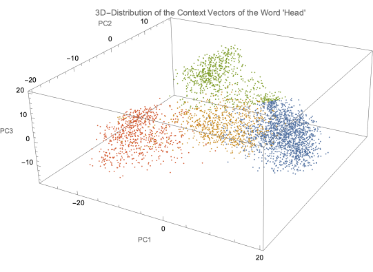
Figure 8. 3D Distribution of the Context Vectors of “Head”
Figure 8 provides a better understanding of the spatial distribution of the vectors. Additionally, the distribution in this diagram is slightly different from the one in Figure 7. In a more detailed study, it would be worth it to analyze these differences to determine how much information is lost between dimensions.
Figure 8 provides a better understanding of the spatial distribution of the vectors. Additionally, the distribution in this diagram is slightly different from the one in Figure 7. In a more detailed study, it would be worth it to analyze these differences to determine how much information is lost between dimensions.
Word “Close”
Word “Close”
The results for “head” are the following:
step1=GetWikiWordText["close",1000];step2=ComputeWordVectors[step1];step3=PlotWordData[step2,2,"Close"]
Out[]=
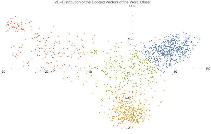
Figure 9. 2D Distribution of the Context Vectors of “Close”
Each point in Figure 9 represents an instance of the word “close” in a Wikipedia sentence. The figure shows that the points form two clusters. The red and green points do not seem to be very related to each other. However, the red points do share a common meaning.
The clusters correspond to the following contexts:
◼
Blue Cluster: Sentences where “close” means intimacy.
◼
Yellow Cluster: Sentences where “close” means proximity.
◼
Red Points: Sentences where “close” means blocking or suspending.
◼
Green Points: Sentences of the three mentioned types.
step1=GetWikiWordText["close",1000];step2=ComputeWordVectors[step1];step3=PlotWordData[step2,3,"Close"]
Out[]=

Figure 10. 3D Distribution of the Context Vectors of “Close”
Figure 10 provides a better understanding of the spatial distribution of the vectors. The distribution resembles that of Figure 4, where one set of points is particularly distant from the others, creating an abrupt separation of context.
Figure 10 provides a better understanding of the spatial distribution of the vectors. The distribution resembles that of Figure 4, where one set of points is particularly distant from the others, creating an abrupt separation of context.
GetWikiWordText
GetWikiWordText
ComputeWordVectors
ComputeWordVectors
PlotWordData
PlotWordData
meanContext
meanContext
Evolution of Interpretation in a Sequence
Evolution of Interpretation in a Sequence
In this experiment I studied how the interpretation of a word changes when processing an increasing sequence. The objective is to better understand the dynamics of the network when deciding the appropriate word vector for the context.
To achieve this, I performed the following procedure:
To achieve this, I performed the following procedure:
1
.Select a word to study and create a sample sentence that includes it. For example:
Word | Run |
Sentence | Irunthegrocerystoredowntheblock. |
2
.Iteratively input the sentence in the ELMo network as an increasing sequence. The sequence starts on the position of the selected word. For example:
1 | Irun |
2 | Irunthe |
3 | Irunthegrocery |
4 | Irunthegrocerystore |
5 | Irunthegrocerystoredown |
6 | Irunthegrocerystoredownthe |
7 | Irunthegrocerystoredowntheblock |
In parallel, save the output vectors corresponding to the word that you are studying.
After performing this step, you must have three vectors per sentence: two contextual and one non-contextual. Every vector has 1024 elements.
After performing this step, you must have three vectors per sentence: two contextual and one non-contextual. Every vector has 1024 elements.
3
.Calculate the mean of the contextual and non-contextual vectors in each sentence.
After performing this step, you must have one vector per sentence, each with 1024 elements.
4
.Reduce the dimensionality of the vectors to two.
After performing this step, you must have one vector per sentence, each with 2 elements.
5
.Plot the vectors against the number of words that the sentence has on each iteration.
I encased this entire process in the ContextEvolution function. To see the implementation details, see the ContextEvolution subsection below.
The plot for the previous example is the following:
The plot for the previous example is the following:
In[]:=
ContextEvolution["I run the grocery store down the block","run"]
Out[]=

Figure 11. Evolution of the Interpretation of the Word “Run” in “I run the grocery store down the block”
Figure 11 shows how the word vector of “run” constantly changes position in the meaning space. When increasing the length of the sequence to “I run the grocery store of my family where I sell apples and bananas”, the plot looks as follows:
ContextEvolution["I run the grocery store down the block where I sell apples and bananas","run"]
Out[]=
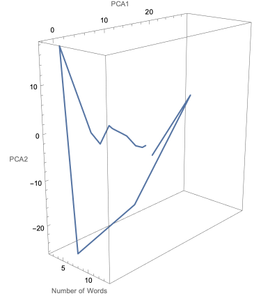
Figure 12. Evolution of the Interpretation of the Word "Run" in "I run the grocery store down the block where I sell apples and bananas"
In Figure 12, the position of the word vector seems to stabilize in a specific region. This could mean that at some point in the sequence, the network has already decided a definition of “run” in this sentence.
In Figure 12, the position of the word vector seems to stabilize in a specific region. This could mean that at some point in the sequence, the network has already decided a definition of “run” in this sentence.
Although the results seem promising, they are not very consistent. In Figures 13 and 14 I analyze the word “play”. For this I compare the plots of the sentences “To play, every player must draw cards every turn and make a move.” and “To play, players are required to draw cards every turn and make a move.”
ContextEvolution["To play every player must draw cards every turn and make a move","play"]
Out[]=

Figure 12. Evolution of the Interpretation of the Word "Run" in "To play, every player must draw cards every turn and make a move"
ContextEvolution["To play, players are required to draw cards every turn and make a move","play"]
Out[]=

Figure 13. Evolution of the Interpretation of the Word "Run" in "To play, players are required to draw cards every turn and make a move"
Even though sentences in Figure 13 and 14 are very similar, their vector trajectories look substantially different. Additionally, the network seems to still be undecided about a definition of the word by the end of the sentence.
ContextEvolution
ContextEvolution
Conclusions
Conclusions
Neural networks like ELMo seem to create their own meaning space structure to identify the meaning of words. This structure is overall efficient, as ELMo can accurately differentiate between contexts.
Acknowledgements
Acknowledgements
I completed this project under the guidance of Connor Gray, who provided great inputsfor the project and also helped me troubleshooting the code.
Tuseeta Banerjee and Jesse Galef also provided initial feedback and structure to the foundations of the project.
Thanks everyone!
Tuseeta Banerjee and Jesse Galef also provided initial feedback and structure to the foundations of the project.
Thanks everyone!
Cite this as: Angelo Barona Balda, "Visualizing Context in the Meaning Space" from the Notebook Archive (2021), https://notebookarchive.org/2021-07-6hpy57e
Download
