Notebook Archive

Browse Categories
About
Contribute

Filter

Apply

Academic Articles & Supplements

The Macrodynamics of an Endogenous Business Cycle Model of Marxist Inspiration

John Cajas Guijarro, Leonardo Vera

Author

John Cajas Guijarro, Leonardo Vera

Title

The Macrodynamics of an Endogenous Business Cycle Model of Marxist Inspiration

Description

Mathematical supplement to accompany Cajas Guijarro and Vera (2022): https://doi.org/10.1016/j.strueco.2022.08.002

Category

Academic Articles & Supplements

Keywords

Business Cycle, Capital Accumulation, Reserve Army of Labor, Labor Intensity, Complex Dynamical Models

URL

http://www.notebookarchive.org/2022-07-b3n4804/

DOI

https://notebookarchive.org/2022-07-b3n4804

Date Added

2022-07-24

Date Last Modified

2022-07-24

File Size

12.74 megabytes

Supplements

Rights

CC BY-NC-SA 4.0

Download

Open in Wolfram Cloud

This file contains supplementary data for John Cajas Guijarro and Leonardo Vera, “The macrodynamics of an endogenous business cycle model of marxist inspiration,” Structural Change and Economic Dynamics, 62, 2022 pp. 566–585. https://doi.org/10.1016/j.strueco.2022.08.002.

(*************************************************************************************************************)(***TheMacrodynamicsofanEndogenousBusinessCycleModelofMarxistInspiration(CajasGuijarroandVera,2022)***)(***************************Source:http://dx.doi.org/10.2139/ssrn.4104317*************************************)(*************************************************************************************************************)

(**Abstract**)(*ThisstudyoffersamodelthatformalizessomeofMarx’sinsightsabouthowcapitalaccumulationgeneratescontradictionsthatmayreproducenever-endingcyclesofboomsandslumps.Themodeltakesthereservearmyoflaborasaregulatorofthedistributionofclass-poweroverthebusinesscyclewithatwo-sidedrole:influencinglaborproductivity,directlythroughtheintensityoflaborandindirectlythroughrealwages.Themodelformsacomplexdynamicalsystemcapabletoyieldtrajectoriesfortheemploymentrate,thewageshare,andtheintensityoflabor.Goodwin(1967)modelmaybeconsideredasaparticularcaseofthemodel.Complexdynamicsmayalsoemergewhenweremovesomekeyassumptionsandexploreandsimulate3-Dversionsofthesystem.Thoughcloseorbitsaroundnon-hyperbolicequilibriumpointscanbeobtained,thepossibilityofunstabledynamicswithincreasingamplitudesinthetradecycleandastructuralcrisiscannotberuledout.*)

In[]:=

ClearAll["Global`*"]

In[]:=

(****Determinantsofcapitalaccumulation****)

In[]:=

eq[2]=k[t]c[t]+ρ*v[t];

In[]:=

eq[3]=c[t]p[t]*A[t];

In[]:=

eq[4]=v[t]w[t]*h*L[t];

In[]:=

eq[5]=Π[t]p[t]*Q[t]-(v[t]+δ*c[t]);

In[]:=

eq[6]=r[t]Π[t]/k[t];

In[]:=

eq[7]=Q[t]q[t]*h*L[t];

In[]:=

eq[8]=m[t]A[t]/L[t];

In[]:=

eq[9]=m'[t]/m[t]γm[t];

In[]:=

eq[10]=q[t]f1[ϵ[t],m[t]];

In[]:=

eq[11]=ω[t]v[t]/(p[t]*Q[t]);

In[]:=

deduction1=Solve[{eq[5],eq[3],eq[4],eq[7],eq[8],eq[11]},{Π[t],c[t],v[t],Q[t],A[t],w[t]}]//FullSimplify

Out[]=

{{Π[t]-L[t]p[t](δm[t]+hq[t](-1+ω[t])),c[t]L[t]m[t]p[t],v[t]hL[t]p[t]q[t]ω[t],Q[t]hL[t]q[t],A[t]L[t]m[t],w[t]p[t]q[t]ω[t]}}

In[]:=

eq[12]=(Solve[deduction1[[1,1,2]]0,ω[t]][[1,1]]//FullSimplify)/.{RuleLess}

Out[]=

ω[t]<1-

δm[t]

hq[t]

In[]:=

eq[13]=k'[t]s*Π[t]-δ*c[t];

In[]:=

eq[14]=γk[t]k'[t]/k[t];

In[]:=

deduction2=Solve[{eq[14],eq[13],eq[6],eq[2],eq[3],eq[4],eq[8],eq[11],eq[7]},{γk[t],k'[t],Π[t],k[t],c[t],v[t],A[t],w[t],Q[t]}]//FullSimplify

Out[]=

γk[t]sr[t]-

δm[t]

m[t]+hρq[t]ω[t]

′

[t]L[t]p[t](m[t](-δ+sr[t])+hsρq[t]r[t]ω[t]),Π[t]L[t]p[t]r[t](m[t]+hρq[t]ω[t]),k[t]L[t]p[t](m[t]+hρq[t]ω[t]),c[t]L[t]m[t]p[t],v[t]hL[t]p[t]q[t]ω[t],A[t]L[t]m[t],w[t]p[t]q[t]ω[t],Q[t]hL[t]q[t]

In[]:=

eq[15]=deduction2[[1,1]]/.{RuleEqual}

Out[]=

γk[t]sr[t]-

δm[t]

m[t]+hρq[t]ω[t]

In[]:=

deduction3=Solve[{eq[6],eq[5],eq[7],eq[2],eq[3],eq[4],eq[8],eq[11]},{r[t],Π[t],Q[t],k[t],c[t],v[t],A[t],w[t]}]//FullSimplify

Out[]=

r[t]-

δm[t]+hq[t](-1+ω[t])

m[t]+hρq[t]ω[t]

,Π[t]-L[t]p[t](δm[t]+hq[t](-1+ω[t])),Q[t]hL[t]q[t],k[t]L[t]p[t](m[t]+hρq[t]ω[t]),c[t]L[t]m[t]p[t],v[t]hL[t]p[t]q[t]ω[t],A[t]L[t]m[t],w[t]p[t]q[t]ω[t]

In[]:=

eq[16]=deduction3[[1,1]]/.{RuleEqual}

Out[]=

r[t]-

δm[t]+hq[t](-1+ω[t])

m[t]+hρq[t]ω[t]

In[]:=

(****Onthereservearmyoflaboranditsmultipleroles****)

In[]:=

eq[17]=l[t]L[t]/NN[t];

In[]:=

eq[18]=NN'[t]/NN[t]n;

In[]:=

deduction4=Solve[{D[eq[17],t],eq[18],eq[17]},{l'[t],NN'[t],NN[t]}]//FullSimplify

Out[]=



′

[t]l[t]-n+

′

[t]

L[t]

′

[t]

nL[t]

l[t]

,NN[t]

L[t]

l[t]



In[]:=

eq[19]=deduction4[[1,1]]/.{RuleEqual}

Out[]=

′

[t]l[t]-n+

′

[t]

L[t]

In[]:=

deduction5=Solve[{eq[8],eq[3],eq[2],eq[4],eq[11],eq[7]},{L[t],A[t],c[t],v[t],w[t],Q[t]}]//FullSimplify

Out[]=

L[t]

k[t]

p[t](m[t]+hρq[t]ω[t])

,A[t]

k[t]m[t]

p[t](m[t]+hρq[t]ω[t])

,c[t]

k[t]m[t]

m[t]+hρq[t]ω[t]

,v[t]

hk[t]q[t]ω[t]

m[t]+hρq[t]ω[t]

,w[t]p[t]q[t]ω[t],Q[t]

hk[t]q[t]

p[t](m[t]+hρq[t]ω[t])



In[]:=

eq[20]=deduction5[[1,1]]/.{RuleEqual}

Out[]=

L[t]

k[t]

p[t](m[t]+hρq[t]ω[t])

In[]:=

deduction6=Solve[{eq[19],D[eq[20],t],eq[20],eq[14],ππ[t]p'[t]/p[t]},{l'[t],L'[t],L[t],k'[t],p'[t]}]//FullSimplify

Out[]=



′

[t]-

m[t]+hρq[t]ω[t]

l[t](m[t](n-γk[t]+ππ[t])+

′

[t]+hρω[t]

′

[t]+hρq[t]((n-γk[t]+ππ[t])ω[t]+

′

[t])),

′

[t]

k[t](m[t](γk[t]-ππ[t])-

′

[t]-hρω[t]

′

[t]+hρq[t]((γk[t]-ππ[t])ω[t]-

′

[t]))

p[t]

(m[t]+hρq[t]ω[t])

,L[t]

k[t]

p[t](m[t]+hρq[t]ω[t])

′

[t]k[t]γk[t],

′

[t]p[t]ππ[t]

In[]:=

eq[21]=Collect[deduction6[[1,1]],{l[t],-γk[t],n,ππ[t]}]/.{RuleEqual}

Out[]=

′

[t]l[t]-n+γk[t]-ππ[t]-

′

[t]+hρω[t]

′

[t]+hρq[t]

′

[t]

m[t]+hρq[t]ω[t]

In[]:=

eq[22]=(w'[t]/w[t]-ππ[t])-α11+α12*l[t]-α13*ππ[t];

In[]:=

eq[23]=ππ[t]α21+α22*l'[t]/l[t]+α23*((w'[t]/w[t])-(q'[t]/q[t]));

In[]:=

eq[24]=ϵ'[t]/ϵ[t]α31-α32*l[t]+α33*(m'[t]/m[t])-α34*ϵ[t]+α35*((w'[t]/w[t])-ππ[t]);

In[]:=

(****Interpretingsomecomplexdynamics****)

In[]:=

deduction7a=Solve[{eq[11],eq[4],eq[7]},{ω[t],v[t],Q[t]}];

In[]:=

deduction7b=deduction7a[[1,1]]/.{RuleEqual}

Out[]=

ω[t]

w[t]

p[t]q[t]

In[]:=

deduction7c=Solve[{eq[21],eq[23],eq[15],eq[16],deduction7b,D[deduction7b,t],ππ[t]p'[t]/p[t]},{l'[t],ππ[t],γk[t],r[t],w[t],w'[t],p'[t]}]//FullSimplify;

In[]:=

eq[25]=Collect[deduction7c[[1,1]]/.{RuleEqual},{l[t],(-1+α23)}]

Out[]=

′

[t]l[t]

(-1+α23)(nm[t]ω[t]+(1+s)δm[t]ω[t]+hsq[t]

ω[t]

+ω[t](

′

[t]+hρω[t]

′

[t]))

(1+α22-α23)ω[t](m[t]+hρq[t]ω[t])

+(-α21m[t]ω[t]+hsq[t]ω[t]-hsα23q[t]ω[t]-h(n+α21)ρq[t]

ω[t]

+hnα23ρq[t]

ω[t]

+(-α23m[t]-hρq[t]ω[t])

′

[t])((1+α22-α23)ω[t](m[t]+hρq[t]ω[t]))

In[]:=

manualeq[25]=l'[t]l[t]*((1-α23)/(1+α22-α23))*(s*((h*(1-ω[t])*q[t]-δ*m[t])/(m[t]+ρ*h*ω[t]*q[t]))-(n+(1/(1-α23))*(α21+α23*ω'[t]/ω[t])+(δ*m[t]+m'[t]+ρ*h*(q[t]*ω'[t]+q'[t]*ω[t]))/(m[t]+ρ*h*ω[t]*q[t])));

In[]:=

(eq[25][[2]]-manualeq[25][[2]])//Simplify

Out[]=

In[]:=

deduction8=Solve[{eq[22],D[deduction7b,t],deduction7b,ππ[t]p'[t]/p[t],eq[23]},{ω'[t],w'[t],w[t],p'[t],ππ[t]}]//FullSimplify;

In[]:=

eq[26]=deduction8[[1,1]]/.{RuleEqual}

Out[]=

′

[t](ω[t](q[t](-l[t](α11+α13α21-α11α23+α12(-1+α23)l[t])-α13α22

′

[t])+(-1+α23)l[t]

′

[t]))/((1+(-1+α13)α23)l[t]q[t])

In[]:=

manualeq[26]=ω'[t]ω[t]*((1-α23)/(1-α23*(1-α13)))*(-α11+α12*l[t]-q'[t]/q[t]-(α13/(1-α23))*(α21+α22*l'[t]/l[t]));

In[]:=

(eq[26][[2]]-manualeq[26][[2]])//Simplify

Out[]=

In[]:=

deduction9=Solve[{eq[24],D[deduction7b,t],deduction7b,ππ[t]p'[t]/p[t]},{ϵ'[t],w'[t],w[t],ππ[t]}]//FullSimplify;

In[]:=

eq[27]=Collect[deduction9[[1,1]]/.{RuleEqual},{ϵ[t],α35}]

Out[]=

′

[t]-α34

ϵ[t]

+ϵ[t]α31-α32l[t]+

α33

′

[t]

m[t]

+α35

′

[t]

q[t]

′

[t]

ω[t]

In[]:=

eq[28]=eq[9]

Out[]=

′

[t]

m[t]

γm[t]

In[]:=

(*****************************************************************)(*****************************ModelA****************************)(*****************************************************************)

In[]:=

caseA={s1,h1,δ0,ρ0,q[t]α40*ϵ[t]*m[t],q'[t]α40*(ϵ'[t]*m[t]+ϵ[t]*m'[t]),α210,α220,α230,α310,α320,α330,α340,α350,ϵ'[t]0,m'[t]m[t]*γm,ϵ[t]ϵ};

In[]:=

{eq[31],eq[32]}=FullSimplify[Solve[({eq[25],eq[26]}/.caseA)/.caseA,{l'[t],ω'[t]}]][[1]]/.{RuleEqual}

Out[]=

{

′

[t]-l[t](n+γm-α40ϵ+α40ϵω[t]),

′

[t]-(α11+γm-α12l[t])ω[t]}

In[]:=

(*ModelA:Equilibrium*)

In[]:=

eq[33]=FullSimplify[Solve[{eq[31],eq[32]}/.{l'[t]0,ω'[t]0},{l[t],ω[t]}]][[2]]/.{RuleEqual}

Out[]=

l[t]

α11+γm

α12

,ω[t]-

n+γm-α40ϵ

α40ϵ



In[]:=

(*ModelA:Stability*)

In[]:=

jacobianA=D[{eq[31][[2]],eq[32][[2]]},{{l[t],ω[t]}}]/.(eq[33]/.{EqualRule})

Out[]=

0,-

α40(α11+γm)ϵ

α12

,-

α12(n+γm-α40ϵ)

α40ϵ

,0

In[]:=

eq[34]={τATr[jacobianA],ΔADet[jacobianA]}//FullSimplify

Out[]=

{τA0,ΔA+(α11+γm)(n+γm-α40ϵ)0}

In[]:=

(*ModelA:Numericalsimulations*)

In[]:=

simulationA1={ϵ1,n0.08,γm0,α110.4,α120.8,α400.2};

In[]:=

simulationA2={ϵ1.25,n0.08,γm0,α110.4,α120.8,α400.2};

In[]:=

solutionA1=NDSolve[{eq[31],eq[32],l[0]0.5,ω[0]0.5}/.simulationA1,{l,ω},{t,0,2000}];

In[]:=

solutionA2=NDSolve[{eq[31],eq[32],l[0]0.5,ω[0]0.5}/.simulationA2,{l,ω},{t,0,2000}];

In[]:=

sollA1=solutionA1[[1,1,2]];

In[]:=

solωA1=solutionA1[[1,2,2]];

In[]:=

sollA2=solutionA2[[1,1,2]];

In[]:=

solωA2=solutionA2[[1,2,2]];

In[]:=

(*ModelA:2DParametricplot*)

In[]:=

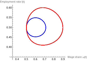
figure1=ParametricPlot[{{solωA1[t],sollA1[t]},{solωA2[t],sollA2[t]}},{t,0,2000},AspectRatio1,AxesLabel{"Wage share ω[t]","Employment rate l[t]"},PlotLegends{"ϵ=1 (A: No inflation)","ϵ=1.25 (A: No inflation)"},AxesOrigin{0.35,0.35},PlotStyle{Blue,Red}]

Out[]=

	ϵ=1 (A: No inflation)
	ϵ=1.25 (A: No inflation)

In[]:=

(*ModelA:Trajectories*)

In[]:=

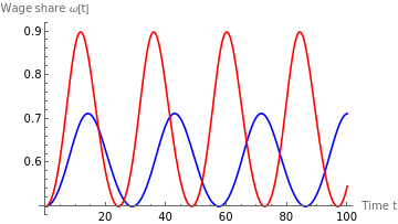
figureB11=Plot[{solωA1[t],solωA2[t]},{t,0,100},AxesLabel{"Time t","Wage share ω[t]"},PlotLegends{"ϵ=1 (A: No inflation)","ϵ=1.25 (A: No inflation)"},PlotStyle{Blue,Red}]

Out[]=

	ϵ=1 (A: No inflation)
	ϵ=1.25 (A: No inflation)

In[]:=

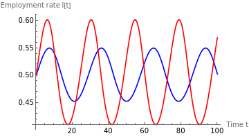
figureB12=Plot[{sollA1[t],sollA2[t]},{t,0,100},AxesLabel{"Time t","Employment rate l[t]"},PlotLegends{"ϵ=1 (A: No inflation)","ϵ=1.25 (A: No inflation)"},PlotStyle{Blue,Red}]

Out[]=

	ϵ=1 (A: No inflation)
	ϵ=1.25 (A: No inflation)

In[]:=

(*****************************************************************)(*****************************ModelB****************************)(*****************************************************************)

In[]:=

caseB={s1,h1,δ0,ρ0,q[t]α40*ϵ[t]*m[t],q'[t]α40*(ϵ'[t]*m[t]+ϵ[t]*m'[t]),α310,α320,α330,α340,α350,ϵ'[t]0,m'[t]m[t]*γm,ϵ[t]ϵ};

In[]:=

{eq[35],eq[36]}=FullSimplify[Solve[({eq[25],eq[26]}/.caseB)/.caseB,{l'[t],ω'[t]}]][[1]]/.{RuleEqual}

Out[]=



′

[t]

1+α22+(-1+α13)α23

(-l[t](n+α21-α11α23+n(-1+α13)α23+γm+(-2+α13)α23γm+(-1+α23-α13α23)α40ϵ+α12α23l[t])+(-1+α23-α13α23)α40ϵl[t]ω[t]),

′

[t]

1+α22+(-1+α13)α23

ω[t](-α13α21+α11(-1-α22+α23)+(-1-α22+α23)γm+α13α22(n+γm-α40ϵ)+α12(1+α22-α23)l[t]+α13α22α40ϵω[t])

In[]:=

(*ModelB:Equilibrium*)

In[]:=

eq[37]=FullSimplify[Solve[{eq[35],eq[36]}/.{l'[t]0,ω'[t]0},{l[t],ω[t]}]][[2]]/.{RuleEqual}

Out[]=

l[t]

α11+α13α21-α11α23+γm-α23γm

α12-α12α23

,ω[t]1-

n+α21-nα23+γm-α23γm

α40ϵ-α23α40ϵ



In[]:=

(*ModelB:Stability*)

In[]:=

jacobianB=D[{eq[35][[2]],eq[36][[2]]},{{l[t],ω[t]}}]/.(eq[37]/.{EqualRule})//FullSimplify

Out[]=



α23(α11+α13α21-α11α23+γm-α23γm)

(-1+α23)(1+α22+(-1+α13)α23)

(-1+α23-α13α23)α40(α11+α13α21-α11α23+γm-α23γm)ϵ

(α12-α12α23)(1+α22+(-1+α13)α23)

,

α12(1+α22-α23)1-

n+α21-nα23+γm-α23γm

α40ϵ-α23α40ϵ



1+α22+(-1+α13)α23

α13α22(n+α21-nα23+γm-α23γm+(-1+α23)α40ϵ)

(-1+α23)(1+α22+(-1+α13)α23)



In[]:=

eq[38]=τBTr[jacobianB]//FullSimplify

Out[]=

τB-((nα13α22(-1+α23)-α13α21(α22+α23)+(-1+α23)α23(α11+γm)+α13α22(-1+α23)(γm-α40ϵ))/((-1+α23)(1+α22+(-1+α13)α23)))

In[]:=

eq[39]=ΔBDet[jacobianB]//FullSimplify

Out[]=

ΔB

(α11+α13α21-α11α23+γm-α23γm)(n+α21-nα23+γm-α23γm+(-1+α23)α40ϵ)

(-1+α23)(1+α22+(-1+α13)α23)

In[]:=

eq[40]=α13B[ϵ](Solve[{eq[38],τB0},{α13,τB}]//FullSimplify)[[1,1,2]]

Out[]=

α13B[ϵ]-

(-1+α23)α23(α11+γm)

nα22(-1+α23)-α21(α22+α23)+α22(-1+α23)(γm-α40ϵ)

In[]:=

eq[41]=ϵB(Solve[{eq[39],ΔB0},{ϵ,ΔB}]//FullSimplify)[[1,1,2]]

Out[]=

ϵB

n+α21-nα23+γm-α23γm

α40-α23α40

In[]:=

(*ModelB:Numericalsimulations*)

In[]:=

simulationB1={ϵ1,n0.08,γm0,α110.4,α120.8,α400.2,α210.01,α220.1,α230.1,α134.09090909};

In[]:=

solutionB1=NDSolve[{eq[35],eq[36],l[0]0.5,ω[0]0.5}/.simulationB1,{l,ω},{t,0,2000}];

In[]:=

sollB1=solutionB1[[1,1,2]];

In[]:=

solωB1=solutionB1[[1,2,2]];

In[]:=

eq[40]/.simulationB1[[2;;10]]

Out[]=

α13B[ϵ]

0.036

-0.0092+0.018ϵ

In[]:=

(*ModelB:stabilityconstraint*)

In[]:=

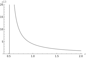
figure2=Plot[eq[40][[2]]/.simulationB1[[2;;10]],{ϵ,0.4,2},PlotRange{0,20},AxesLabel{"ϵ","α13"},PlotStyleGray]

Out[]=

In[]:=

(*ModelAvsModelB:2DParametricplot*)

In[]:=

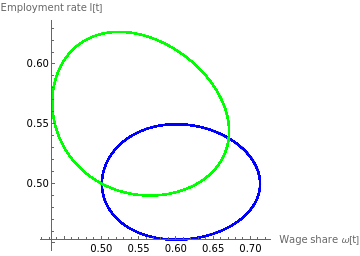
figure3=ParametricPlot[{{solωA1[t],sollA1[t]},{solωB1[t],sollB1[t]}},{t,0,2000},AspectRatio1,AxesLabel{"Wage share ω[t]","Employment rate l[t]"},PlotStyle{Blue,Green},PlotLegends{"ϵ=1 (A: No inflation)","ϵ=1 (B: Endogenous inflation)"}]

Out[]=

	ϵ=1 (A: No inflation)
	ϵ=1 (B: Endogenous inflation)

In[]:=

(*ModelAvsModelB:Trajectories*)

In[]:=

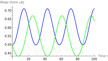
figureB21=Plot[{solωA1[t],solωB1[t]},{t,0,100},AxesLabel{"Time t","Wage share ω[t]"},PlotLegends{"ϵ=1 (A: No inflation)","ϵ=1 (B: Endogenous inflation)"},PlotStyle{Blue,Green}]

Out[]=

	ϵ=1 (A: No inflation)
	ϵ=1 (B: Endogenous inflation)

In[]:=

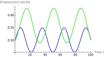
figureB22=Plot[{sollA1[t],sollB1[t]},{t,0,100},AxesLabel{"Time t","Employment rate l[t]"},PlotLegends{"ϵ=1 (A: No inflation)","ϵ=1 (B: Endogenous inflation)"},PlotStyle{Blue,Green}]

Out[]=

	ϵ=1 (A: No inflation)
	ϵ=1 (B: Endogenous inflation)

In[]:=

(*****************************************************************)(*****************************ModelC****************************)(*****************************************************************)

In[]:=

caseC={s1,h1,δ0,ρ0,q[t]α40*ϵ[t]*m[t],q'[t]α40*(ϵ'[t]*m[t]+ϵ[t]*m'[t]),α210,α220,α230,m'[t]m[t]*0,γm0};

In[]:=

{eq[42],eq[43],eq[44]}=FullSimplify[Solve[({eq[25],eq[26],eq[27]}/.caseC)/.caseC,{l'[t],ω'[t],ϵ'[t]}]][[1]]/.{RuleEqual}

Out[]=

{

′

[t]-l[t](n+α40ϵ[t](-1+ω[t])),

′

[t](-α31+α11(-1+α35)+(α12+α32-α12α35)l[t]+α34ϵ[t])ω[t],

′

[t]ϵ[t](α31-α11α35+(-α32+α12α35)l[t]-α34ϵ[t])}

In[]:=

(*ModelC:Equilibrium*)

In[]:=

eq[45]=FullSimplify[Solve[{eq[42],eq[43],eq[44]}/.{l'[t]0,ω'[t]0,ϵ'[t]0},{l[t],ω[t],ϵ[t]}]][[2]]/.{RuleEqual}

Out[]=

l[t]

α11

α12

,ω[t]1-

nα12α34

α12α31α40-α11α32α40

,ϵ[t]

α12α31-α11α32

α12α34



In[]:=

(*ModelC:Stability(seeAppendixA.1)*)

In[]:=

jacobianC=D[{eq[42][[2]],eq[43][[2]],eq[44][[2]]},{{l[t],ω[t],ϵ[t]}}]/.(eq[45]/.{EqualRule})//FullSimplify

Out[]=

0,

α11(-α12α31+α11α32)α40

α12

α34

nα11α34

α12α31-α11α32

,(α12+α32-α12α35)1-

nα12α34

α12α31α40-α11α32α40

,0,α341-

nα12α34

α12α31α40-α11α32α40

,

(α12α31-α11α32)(-α32+α12α35)

α12α34

,0,-α31+

α11α32

α12



In[]:=

charpolinomialC=Collect[FullSimplify[CharacteristicPolynomial[jacobianC,λ]],λ]

Out[]=

nα11

α12

α31α34-n

α11

α12α32α34-α11

(α12α31-α11α32)

α40

α12

α34

(nα11

α12

α34+α11(α12α31-α11α32)(-α32+α12(-1+α35))α40)λ

α12

α34

(-α12α31+α11α32)

α12

In[]:=

eqb1C=b1[α32](-Tr[jacobianC]//FullSimplify)

Out[]=

b1[α32]α31-

α11α32

α12

In[]:=

eqb2C=b2[α32](Tr[Minors[jacobianC]]//FullSimplify)

Out[]=

b2[α32]-nα11+

α11(-α12α31+α11α32)(-α32+α12(-1+α35))α40

α12

α34

In[]:=

eqb3C=b3[α32](-Det[jacobianC]//FullSimplify)

Out[]=

b3[α32]

α11(-α12α31+α11α32)(nα12α34-α12α31α40+α11α32α40)

α12

α34

In[]:=

eqb123C=b1[α32]*b2[α32]-b3[α32]((eqb1C[[2]]*eqb2C[[2]]-eqb3C[[2]])//FullSimplify)

Out[]=

b1[α32]b2[α32]-b3[α32]-

α11

(α12α31-α11α32)

(-α32+α12α35)α40

α12

α34

In[]:=

criticalvalC=Solve[eqb123C[[2]]0,α32]

Out[]=

α32

α12α31

α11

,α32

α12α31

α11

,{α32α12α35}

In[]:=

(*ModelC:Hopfbifurcation(seeAppendixA.2)*)

In[]:=

Hopf1=criticalvalC[[3,1]]/.{RuleEqual}

Out[]=

α32α12α35

In[]:=

eqdb1C=FullSimplify[D[eqb1C,α32]]

Out[]=

α11

α12

′

[α32]0

In[]:=

eqdb2C=FullSimplify[D[eqb2C,α32]]

Out[]=

′

[α32]

α11(α12α31-2α11α32+α11α12(-1+α35))α40

α12

α34

In[]:=

eqdb3C=FullSimplify[D[eqb3C,α32]]

Out[]=

′

[α32]

α11

(nα12α34-2α12α31α40+2α11α32α40)

α12

α34

In[]:=

HopfsistemC=Solve[{eqdb1C,eqdb2C,eqdb3C,-X-2*Yb1'[α32],2*λ1*Y+2*b*Zb2'[α32],-b*b*X-2*λ1*b*Zb3'[α32]},{b1'[α32],b2'[α32],b3'[α32],X,Y,Z}]//FullSimplify

Out[]=



′

[α32]-

α11

α12

′

[α32]

α11(α12α31-2α11α32+α11α12(-1+α35))α40

α12

α34

′

[α32]

α11

(nα12α34-2α12α31α40+2α11α32α40)

α12

α34

,X

α12

α34(

λ1

)

α11(-nα11α12α34+2α11(α12α31-α11α32)α40+(-α12α31+α11(α12+2α32-α12α35))α40λ1+α12α34

λ1

),Y

α12

α34(

λ1

)

α11(

α12α34+α11(nα12α34-2α12α31α40+2α11α32α40)+(α12α31-2α11α32+α11α12(-1+α35))α40λ1),Z-

α12

α34(

λ1

)

α11(α11(nα12α34-2α12α31α40+2α11α32α40)λ1+

(-α12α31α40+α11(α12+2α32-α12α35)α40+α12α34λ1))

In[]:=

Hopf2=((HopfsistemC[[1,5]]/.{Hopf1/.{EqualRule}})//FullSimplify)/.{RuleEqual}

Out[]=

Y

α11(

α34+nα11α34+α40(2

α11

α35+α31λ1-α11(2α31+λ1+α35λ1)))

2α12α34(

λ1

)

In[]:=

(*ModelC:Numericalsimulations*)

In[]:=

simulationC1={n0.08,α110.4,α120.8,α400.2,α310.1,α320.08001,α330.1,α340.05,α350.1};

In[]:=

solutionC11=NDSolve[{eq[42],eq[43],eq[44],l[0]0.5,ω[0]0.5,ϵ[0]0.7}/.simulationC1,{l,ω,ϵ},{t,0,2000}];

In[]:=

solutionC12=NDSolve[{eq[42],eq[43],eq[44],l[0]0.5,ω[0]0.5,ϵ[0]1}/.simulationC1,{l,ω,ϵ},{t,0,2000}];

In[]:=

solutionC13=NDSolve[{eq[42],eq[43],eq[44],l[0]0.5,ω[0]0.5,ϵ[0]1.25}/.simulationC1,{l,ω,ϵ},{t,0,2000}];

In[]:=

solutionC14=NDSolve[{eq[42],eq[43],eq[44],l[0]0.5,ω[0]0.5,ϵ[0]1.5}/.simulationC1,{l,ω,ϵ},{t,0,2000}];

In[]:=

sollC11=solutionC11[[1,1,2]];

In[]:=

solωC11=solutionC11[[1,2,2]];

In[]:=

solϵC11=solutionC11[[1,3,2]];

In[]:=

sollC12=solutionC12[[1,1,2]];

In[]:=

solωC12=solutionC12[[1,2,2]];

In[]:=

solϵC12=solutionC12[[1,3,2]];

In[]:=

sollC13=solutionC13[[1,1,2]];

In[]:=

solωC13=solutionC13[[1,2,2]];

In[]:=

solϵC13=solutionC13[[1,3,2]];

In[]:=

sollC14=solutionC14[[1,1,2]];

In[]:=

solωC14=solutionC14[[1,2,2]];

In[]:=

solϵC14=solutionC14[[1,3,2]];

In[]:=

(*ModelC:2Dand3Dparametricplotswithdifferentinitialvaluesforϵ*)

In[]:=

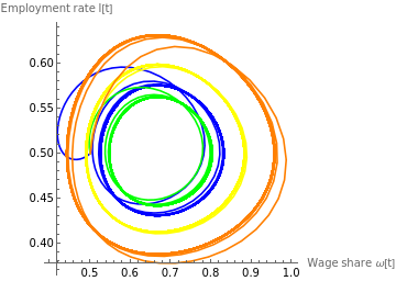
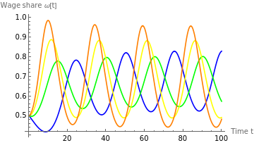
figure4a=ParametricPlot[{{solωC11[t],sollC11[t]},{solωC12[t],sollC12[t]},{solωC13[t],sollC13[t]},{solωC14[t],sollC14[t]}},{t,0,2000},AspectRatio1,AxesLabel{"Wage share ω[t]","Employment rate l[t]"},PlotStyle{Blue,Green,Yellow,Orange},PlotLegends{"ϵ[0]=0.7","ϵ[0]=1","ϵ[0]=1.25","ϵ[0]=1.5"}]

Out[]=

	ϵ[0]=0.7
	ϵ[0]=1
	ϵ[0]=1.25
	ϵ[0]=1.5

In[]:=

figure4b=ParametricPlot3D[{{solωC11[t],sollC11[t],solϵC11[t]},{solωC12[t],sollC12[t],solϵC12[t]},{solωC13[t],sollC13[t],solϵC13[t]},{solωC14[t],sollC14[t],solϵC14[t]}},{t,0,800},AxesLabel{"Wage share ω[t]","Employment rate l[t]","Labour intensity ϵ[t]"},PlotStyle{Blue,Green,Yellow,Orange},PlotRange{{0.3,1},{0.35,0.7},{0.8,1.6}},PlotLegends{"ϵ[0]=0.7","ϵ[0]=1","ϵ[0]=1.25","ϵ[0]=1.5"}]

Out[]=

	ϵ[0]=0.7
	ϵ[0]=1
	ϵ[0]=1.25
	ϵ[0]=1.5

(*ModelC:Alternative3Dparametricplot*)

In[]:=

initialvalC1=Table[{0.5,0.5,x},{x,0.8,1.5,0.025}];

In[]:=

complex3D[eq1_,eq2_,eq3_,t_,ω0_,l0_,ϵ0_,simulation_]:=Block[{ω,l,ϵ},Evaluate[{ω[t],l[t],ϵ[t]}/.NDSolve[{eq1,eq2,eq3,ω[0]ω0,l[0]l0,ϵ[0]ϵ0}/.simulation,{l,ω,ϵ},{t,0,2000}]]]

In[]:=

figure4c=ParametricPlot3D[Evaluate[Table[complex3D[eq[42],eq[43],eq[44],t,x[[1]],x[[2]],x[[3]],simulationC1],{x,initialvalC1}]],{t,0,2000},PlotRange{{0.3,1},{0.35,0.7},{0.8,1.6}},AxesLabel{"Wage share ω[t]","Employment rate l[t]","Labour intensity ϵ[t]"}]

Out[]=

(*ModelC:Trajectories*)

In[]:=

figureB31=Plot[{solωC11[t],solωC12[t],solωC13[t],solωC14[t]},{t,0,100},AxesLabel{"Time t","Wage share ω[t]"},PlotLegends{"ϵ=0.75","ϵ=1","ϵ=1.25","ϵ=1.75"},PlotStyle{Blue,Green,Yellow,Orange}]

Out[]=

	ϵ=0.75
	ϵ=1
	ϵ=1.25
	ϵ=1.75

In[]:=

figureB32=Plot[{sollC11[t],sollC12[t],sollC13[t],sollC14[t]},{t,0,100},AxesLabel{"Time t","Rate of employment l[t]"},PlotLegends{"ϵ=0.75","ϵ=1","ϵ=1.25","ϵ=1.75"},PlotStyle{Blue,Green,Yellow,Orange}]

Out[]=

	ϵ=0.75
	ϵ=1
	ϵ=1.25
	ϵ=1.75

In[]:=

figureB33=Plot[{solϵC11[t],solϵC12[t],solϵC13[t],solϵC14[t]},{t,0,100},AxesLabel{"Time t","Labour intensity ϵ[t]"},PlotLegends{"ϵ=0.75","ϵ=1","ϵ=1.25","ϵ=1.75"},PlotStyle{Blue,Green,Yellow,Orange},PlotRangeAll]

Out[]=

	ϵ=0.75
	ϵ=1
	ϵ=1.25
	ϵ=1.75

(*ModelC:Stablespiralsforthetrajectoryofthelaborintensity*)

In[]:=

simulationC2={n0.08,α110.4,α120.8,α400.2,α310.1,α320.08001+0.03,α330.1,α340.05,α350.1};

In[]:=

solutionC21=NDSolve[{eq[42],eq[43],eq[44],l[0]0.5,ω[0]0.5,ϵ[0]1}/.simulationC2,{l,ω,ϵ},{t,0,2000}];

In[]:=

sollC21=solutionC21[[1,1,2]];

In[]:=

solωC21=solutionC21[[1,2,2]];

In[]:=

solϵC21=solutionC21[[1,3,2]];

In[]:=

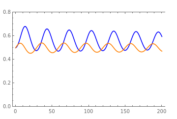
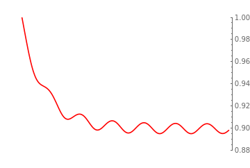
figure5a=Overlay[{Plot[{solωC21[t],sollC21[t]},{t,0,200},AxesLabel{"Time t"},PlotLegends{"Wage share ω[t]","Employment rate l[t]"},PlotStyle{Blue,Orange},PlotRange{0,0.8},Frame{True,True,True,False},ImagePadding25],Plot[{solϵC21[t]},{t,0,200},AxesLabel{"Time t"},PlotLegends{"Labor intensity ϵ[t]"},PlotStyleRed,PlotRange{0.88,1},Frame{False,False,False,True},ImagePadding25,FrameTicks{{None,All},{None,None}}]}]

Out[]=

	Wage share ω[t]
	Employment rate l[t]

Labor intensity ϵ[t]

In[]:=

initialvalC2=Table[{0.5,0.5,x},{x,0.8,1.5,0.025}];

In[]:=

figure5b=ParametricPlot3D[Evaluate[Table[complex3D[eq[42],eq[43],eq[44],t,x[[1]],x[[2]],x[[3]],simulationC2],{x,initialvalC2}]],{t,0,2000},PlotRange{{0.3,1},{0.35,0.7},{0.8,1.6}},AxesLabel{"Wage share ω[t]","Employment rate l[t]","Labour intensity ϵ[t]"}]

Out[]=

(*ModelC:Limitcycleswithmultipleinitialvaluesforωandl*)

In[]:=

solutionC15=NDSolve[{eq[42],eq[43],eq[44],l[0]0.5,ω[0]0.5,ϵ[0]1}/.simulationC1,{l,ω,ϵ},{t,0,2000}];

In[]:=

solutionC16=NDSolve[{eq[42],eq[43],eq[44],l[0]0.5,ω[0]0.3,ϵ[0]1}/.simulationC1,{l,ω,ϵ},{t,0,2000}];

In[]:=

solutionC17=NDSolve[{eq[42],eq[43],eq[44],l[0]0.6,ω[0]0.4,ϵ[0]1}/.simulationC1,{l,ω,ϵ},{t,0,2000}];

In[]:=

solutionC18=NDSolve[{eq[42],eq[43],eq[44],l[0]0.7,ω[0]0.5,ϵ[0]1}/.simulationC1,{l,ω,ϵ},{t,0,2000}];

In[]:=

sollC15=solutionC15[[1,1,2]];

In[]:=

solωC15=solutionC15[[1,2,2]];

In[]:=

solϵC15=solutionC15[[1,3,2]];

In[]:=

sollC16=solutionC16[[1,1,2]];

In[]:=

solωC16=solutionC16[[1,2,2]];

In[]:=

solϵC16=solutionC16[[1,3,2]];

In[]:=

sollC17=solutionC17[[1,1,2]];

In[]:=

solωC17=solutionC17[[1,2,2]];

In[]:=

solϵC17=solutionC17[[1,3,2]];

In[]:=

sollC18=solutionC18[[1,1,2]];

In[]:=

solωC18=solutionC18[[1,2,2]];

In[]:=

solϵC18=solutionC18[[1,3,2]];

In[]:=

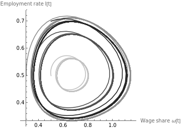
figure6=ParametricPlot[{{solωC15[t],sollC15[t]},{solωC16[t],sollC16[t]},{solωC17[t],sollC17[t]},{solωC18[t],sollC18[t]}},{t,0,2000},AspectRatio1,AxesLabel{"Wage share ω[t]","Employment rate l[t]"},PlotStyle{GrayLevel[0.76],GrayLevel[0.57],GrayLevel[0.32],GrayLevel[0.16]},PlotLegends{"ω[0]=0.5, l[0]=0.5, ϵ[0]=1","ω[0]=0.3, l[0]=0.5, ϵ[0]=1","ω[0]=0.4, l[0]=0.6, ϵ[0]=1","ω[0]=0.5, l[0]=0.7, ϵ[0]=1"}]

Out[]=

	ω[0]=0.5, l[0]=0.5, ϵ[0]=1
	ω[0]=0.3, l[0]=0.5, ϵ[0]=1
	ω[0]=0.4, l[0]=0.6, ϵ[0]=1
	ω[0]=0.5, l[0]=0.7, ϵ[0]=1

(*****************************************************************)(*****************************ModelD****************************)(*****************************************************************)

In[]:=

caseD={s1,h1,δ0,ρ0,q[t]α40*ϵ[t]*m[t],q'[t]α40*(ϵ'[t]*m[t]+ϵ[t]*m'[t]),m'[t]m[t]*γm};

In[]:=

eq[48]=FullSimplify[Solve[({eq[25],eq[26],eq[27]}/.caseD)/.caseD,{l'[t],ω'[t],ϵ'[t]}]][[1]]/.{RuleEqual}

Out[]=



′

[t]

1+α22+α23(-1+α13-α13α35)

l[t](-α21+n(-1+α23+α13α23(-1+α35))-γm+α23(α11+α31-α11α35+(2+α33+α13(-1+α35))γm)-α23(α12+α32-α12α35)l[t]+ϵ[t](α40-α23(α34+α40+α13(-1+α35)α40)+(-1+α23+α13α23(-1+α35))α40ω[t])),

′

[t]-

1+α22+α23(-1+α13-α13α35)

ω[t](-α11(1+α22-α23)(-1+α35)+(1+α22-α23)(α31+γm+α33γm)-α13(-1+α35)(α21-α22(n+γm))-(1+α22-α23)(α12+α32-α12α35)l[t]-α34ϵ[t]+ϵ[t](α23α34-α22(α34+α13(-1+α35)α40)+α13α22(-1+α35)α40ω[t])),

′

[t]

1+α22+α23(-1+α13-α13α35)

ϵ[t]((1+α22+(-1+α13)α23)α31-(α13(α21-nα22)+α11(1+α22-α23))α35+(1+α22+(-1+α13)α23)α33γm+α13(α22+α23)α35γm-((1+α22+(-1+α13)α23)α32+α12(-1-α22+α23)α35)l[t]-ϵ[t]((1+α22+(-1+α13)α23)α34+α13α22α35α40-α13α22α35α40ω[t]))

(*ModelD:Equilibrium*)

In[]:=

{eq[49],eq[50],eq[51]}=FullSimplify[Solve[eq[48]/.{l'[t]0,ω'[t]0,ϵ'[t]0},{l[t],ω[t],ϵ[t]}]][[4]]/.{RuleEqual}

Out[]=

l[t]

α11+α13α21-α11α23+γm-α23γm

α12-α12α23

,ω[t](α12α21α34-nα12(-1+α23)α34+α32α40(α11+α13α21-α11α23+γm-α23γm)+α12(-1+α23)(-α34γm+α40(α31+(α33+α35)γm)))(α40(α32(α11+α13α21-α11α23+γm-α23γm)+α12(-1+α23)(α31+(α33+α35)γm))),ϵ[t]

α31+

-α11α32+

α13α21α32

-1+α23

-α32γm+α12(α33+α35)γm

α12

α34



(*ModelD:Stabilityanalysisusingnumericalsimulations*)

In[]:=

simulationD1={n0.08,γm0,α110.4,α120.8,α400.2,α210.01,α220.1,α230.1,α310.1,α330.1,α340.05,α350.1,α13α13,α32α32};

In[]:=

jacobianD=D[{eq[48][[1,2]],eq[48][[2,2]],eq[48][[3,2]]},{{l[t],ω[t],ϵ[t]}}]/.({eq[49],eq[50],eq[51]}/.{EqualRule})//FullSimplify;

In[]:=

jacobianD1=(jacobianD/.simulationD1)//FullSimplify;

In[]:=

eqb1D=b1[α32](-Tr[jacobianD1]//FullSimplify);

In[]:=

eqb2D=b2[α32](Tr[Minors[jacobianD1]]//FullSimplify);

In[]:=

eqb3D=b3[α32](-Det[jacobianD1]//FullSimplify);

In[]:=

eqb123D=b1[α32]*b2[α32]-b3[α32]((eqb1D[[2]]*eqb2D[[2]]-eqb3D[[2]])//FullSimplify);

In[]:=

fcriticalvalD[valα13_]:={valα13,If[Solve[(eqb123D[[2]]/.{α13valα13})0,α32][[1,1,2]]>0,Solve[(eqb123D[[2]]/.{α13valα13})0,α32][[1,1,2]],Solve[(eqb123D[[2]]/.{α13valα13})0,α32][[2,1,2]]]}

In[]:=

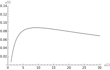
figure8=ListLinePlot[Table[fcriticalvalD[x],{x,1,30,0.25}],PlotMarkers{Automatic,4},PlotRange{0,0.14},AxesLabel{"α13","α32"},PlotStyleGray]

Solve

:Solve was unable to solve the system with inexact coefficients. The answer was obtained by solving a corresponding exact system and numericizing the result.

Solve

:Solve was unable to solve the system with inexact coefficients. The answer was obtained by solving a corresponding exact system and numericizing the result.

Solve

:Solve was unable to solve the system with inexact coefficients. The answer was obtained by solving a corresponding exact system and numericizing the result.

General

:Further output of Solve::ratnz will be suppressed during this calculation.

Out[]=

(*ModelD:Simulationsand3Dparametricplot*)

In[]:=

simulationsD=Table[{n0.08,γm0,α110.4,α120.8,α400.2,α210.01,α220.1,α230.1,α310.1,α330.1,α340.05,α350.1,α13x,α32fcriticalvalD[x][[2]]},{x,1.5,16,0.25}];

Solve

:Solve was unable to solve the system with inexact coefficients. The answer was obtained by solving a corresponding exact system and numericizing the result.

Solve

:Solve was unable to solve the system with inexact coefficients. The answer was obtained by solving a corresponding exact system and numericizing the result.

Solve

:Solve was unable to solve the system with inexact coefficients. The answer was obtained by solving a corresponding exact system and numericizing the result.

General

:Further output of Solve::ratnz will be suppressed during this calculation.

In[]:=

figure7=Show[ParametricPlot3D[Evaluate[Table[complex3D[eq[48][[1]],eq[48][[2]],eq[48][[3]],t,0.5,0.5,1,x],{x,simulationsD}]],{t,0,2000},PlotRange{{0,1},{0,1},{0.5,2}},AxesLabel{"Wage share ω[t]","Employment rate l[t]","Labour intensity ϵ[t]"}],Graphics3D[{PointSize[0.02],Black,Point[{0.5,0.5,1}]}]]

Out[]=

Cite this as: John Cajas Guijarro, Leonardo Vera, "The Macrodynamics of an Endogenous Business Cycle Model of Marxist Inspiration" from the Notebook Archive (2022), https://notebookarchive.org/2022-07-b3n4804

Wolfram Foundation

Download