Implementation of a generalized method of image dyons for quasi-two dimensional slabs with ordinary - topological insulator interfaces
Author
Jose L. Movilla, Juan I. Climente, Josep Planelles
Title
Implementation of a generalized method of image dyons for quasi-two dimensional slabs with ordinary - topological insulator interfaces
Description
Implementation of a generalized method of image dyons for quasi-two dimensional slabs with ordinary - topological insulator interfaces
Category
Academic Articles & Supplements
Keywords
Topological insulator, Magnetoelectrics, Image dyon method, Quantum well
URL
http://www.notebookarchive.org/2023-02-45ox0tv/
DOI
https://notebookarchive.org/2023-02-45ox0tv
Date Added
2023-02-09
Date Last Modified
2023-02-09
File Size
457.82 kilobytes
Supplements
Rights
CC BY 4.0

This file contains supplementary material for J. L. Movilla, J. I. Climente, and J. Planelles, “Generalized method of image dyons for quasi-two dimensional slabs with ordinary - topological insulator interfaces”, in preparation.
Implementation of a generalized method of image dyons for quasi-two dimensional slabs with ordinary - topological insulator interfaces
Implementation of a generalized method of image dyons for quasi-two dimensional slabs with ordinary - topological insulator interfaces
Jose L. Movilla (a), Juan I. Climente (b), Josep Planelles (b)
(a) Dept. d’Educació i Didàctiques Específiques, Universitat Jaume I, 12080, Castelló, Spain
(b) Dept. de Química Física i Analítica, Universitat Jaume I, 12080, Castelló, Spain
Electrostatic charges near the interface bewteen topological (TI) and ordinary (OI) insulators induce magnetic fields in the medium that can be described through the so-called method of image dyons (electric charge - magnetic monopole pairs), the magnetoelectric extension of the method of image charges in classical electrostatics. In this code we calculate recurrently the image dyons and ensuing magnetoelectric potentials in a system comprised by two planar-parallel OI-TI interfaces conforming a finite-width slab, in order to model magnetoelectric fields in topological quantum wells, thin films, or layers of two-dimensional materials.
Electrostatic charges near the interface bewteen topological (TI) and ordinary (OI) insulators induce magnetic fields in the medium that can be described through the so-called method of image dyons (electric charge - magnetic monopole pairs), the magnetoelectric extension of the method of image charges in classical electrostatics. In this code we calculate recurrently the image dyons and ensuing magnetoelectric potentials in a system comprised by two planar-parallel OI-TI interfaces conforming a finite-width slab, in order to model magnetoelectric fields in topological quantum wells, thin films, or layers of two-dimensional materials.
System and input parameters
System and input parameters
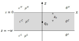
The modelled system and related parameters are sketched in the figure: a electrostatic charge q0 is placed on top or inside a w-width slab with OI-TI interfaces. We assume that:
- The upper (U) interface is located at z = 0.
- The lower (L) inteface is located at z = -w.
- q0 is located along the z axis.
- We have either a TI slab between two OI [i.e., (θU,θC,θL)=(0,π,0)], or a OI slab between two TI [i.e., (θU,θC,θL)=(π,0,π)].
- The upper (U) interface is located at z = 0.
- The lower (L) inteface is located at z = -w.
- q0 is located along the z axis.
- We have either a TI slab between two OI [i.e., (θU,θC,θL)=(0,π,0)], or a OI slab between two TI [i.e., (θU,θC,θL)=(π,0,π)].
The input parameters are(*):
- q0: electrostatic point charge.
- z0: absolute value of the position of q0 in the z axis.
- w: width of the slab.
- α: Fine structure constant.
- Dielectric constants: ϵU (z>0), ϵC (0>z>-w), ϵL (-w>z)
- Magnetic permeabilities: μU (z>0), μC (0>z>-w), μL (-w>z)
- kmax: Cutoff of the otherwise infinite series in the calculation of the magnetoelectric potentials.
- location: Position of q0: “in” (in the C medium) or “out” (in the U medium).
- (*) All input parameters must be expressed in Gaussian atomic units.
ClearAll["Global`*"]
(*Unitsconversionparameters*)elv=27.211386246;(*electron-volts/a.u.*)ban=0.529177210903*10^-10;(*meters/a.u.*)teslaG=1.71525554109*10^3;(*tesla/a.u.(intheGaussianconvention)*)alpha=1/137.036;(*Finestructureconstant*)
(************************INPUTDATA***********************)(*InputdataforMaterials'parameters(ina.u.):*)dataM={ϵU1,ϵC10,ϵL5,μU1,μC1,μL1,αalpha,q01,ηU1,ηL1};(*InputdataforStructureparameters(ina.u.):*)dataS={w10*10^-9/ban,z05*10^-9/ban};(*Cutoffoftheotherwiseinfiniteseries:*)kmax=100;(*Selectthelocationofthesourcechargeq0*)location="in";(*"in"forq0insidetheslab."out"forq0outside(ontopof)theslab.*)(*******************ENDOFINPUTDATA*********************)
(*Definelq0(auxiliaryparameterrelatedtothelocationofq0insideoroutsidetheslab)*)lq0=Which[location"out",1,location"in",-1,True,Print["Warning: position must be 'in' or 'out'"]];
(*Dyonspositioninthezaxis*)zkν[k_,ν_,z0_,w_]:=νSign[k](z0+2(k-Sign[k])w);
(*Particularizationoftheelectricchargesandmagneticmonopolesforthematerials'parametersindataM*)i=1;qUkν[i,1]=qUkν[i,1]/.dataM;qUkν[i,-1]=qUkν[i,-1]/.dataM;gUkν[i,1]=gUkν[i,1]/.dataM;gUkν[i,-1]=gUkν[i,-1]/.dataM;qLkν[i,1]=qLkν[i,1]/.dataM;gLkν[i,1]=gLkν[i,1]/.dataM;For[i=2,i≤kmax,i++,qUkν[i,1]=qUkν[i,1]/.dataM;qUkν[i,-1]=qUkν[i,-1]/.dataM;gUkν[i,1]=gUkν[i,1]/.dataM;gUkν[i,-1]=gUkν[i,-1]/.dataM;qLkν[i,1]=qLkν[i,1]/.dataM;qLkν[i,-1]=qLkν[i,-1]/.dataM;gLkν[i,1]=gLkν[i,1]/.dataM;gLkν[i,-1]=gLkν[i,-1]/.dataM;]If[lq0-1,(*ifq0in-z0/0>-z0>-w*)i=-1;qLmkν[i,1]=qLmkν[i,1]/.dataM;gLmkν[i,1]=gLmkν[i,1]/.dataM;For[i=2,i≤kmax,i++,qUmkν[-i,1]=qUmkν[-i,1]/.dataM;qUmkν[-i,-1]=qUmkν[-i,-1]/.dataM;gUmkν[-i,1]=gUmkν[-i,1]/.dataM;gUmkν[-i,-1]=gUmkν[-i,-1]/.dataM;qLmkν[-i,1]=qLmkν[-i,1]/.dataM;qLmkν[-i,-1]=qLmkν[-i,-1]/.dataM;gLmkν[-i,1]=gLmkν[-i,1]/.dataM;gLmkν[-i,-1]=gLmkν[-i,-1]/.dataM;];];
(*DEFININGTHEFIELDS*)zz0=z0/.dataS;(*Absolutevalueofthelocationofq0inthezaxis.(Theactuallocationofq0is(0,0,lq0*zz0))*)ww=w/.dataS;(*Widthoftheslab*)(*DefiningtheELECTRICFIELD*)dxzVUz[x_,z_]=-VU[x,z,0,zz0,ww];dxzVCz[x_,z_]=-VC[x,z,0,zz0,ww];dxzVLz[x_,z_]=-VL[x,z,0,zz0,ww];dxzVUx[x_,z_]=-VU[x,z,0,zz0,ww];dxzVCx[x_,z_]=-VC[x,z,0,zz0,ww];dxzVLx[x_,z_]=-VL[x,z,0,zz0,ww];Efield[x_,z_]=Piecewise[{{{dxzVUx[x,z],dxzVUz[x,z]},z≥0},{{dxzVCx[x,z],dxzVCz[x,z]},0>z>-ww},{{dxzVLx[x,z],dxzVLz[x,z]},z≤-ww}}];(*DefiningtheMAGNETICFIELD*)dxzUUz[x_,z_]=-UU[x,z,0,zz0,ww];dxzUCz[x_,z_]=-UC[x,z,0,zz0,ww];dxzULz[x_,z_]=-UL[x,z,0,zz0,ww];dxzUUx[x_,z_]=-UU[x,z,0,zz0,ww];dxzUCx[x_,z_]=-UC[x,z,0,zz0,ww];dxzULx[x_,z_]=-UL[x,z,0,zz0,ww];Bfield[x_,z_]=Piecewise[{{{dxzUUx[x,z],dxzUUz[x,z]},z≥0},{{dxzUCx[x,z],dxzUCz[x,z]},0>z>-ww},{{dxzULx[x,z],dxzULz[x,z]},z≤-ww}}];
∂
z
∂
z
∂
z
∂
x
∂
x
∂
x
∂
z
∂
z
∂
z
∂
x
∂
x
∂
x
(******EXAMPLEPLOTS******)
(*DefiningtheMAGNETICFIELDinmiliteslaandthelengthparametersinnanometers*)BfieldnmmT[x_,z_]=Piecewise[{{{teslaG*1000*dxzUUx[x*10^-9/ban,z*10^-9/ban],teslaG*1000*dxzUUz[x*10^-9/ban,z*10^-9/ban]},z≥0},{{teslaG*1000*dxzUCx[x*10^-9/ban,z*10^-9/ban],teslaG*1000*dxzUCz[x*10^-9/ban,z*10^-9/ban]},0>z*10^-9/ban>-ww},{{teslaG*1000*dxzULx[x*10^-9/ban,z*10^-9/ban],teslaG*1000*dxzULz[x*10^-9/ban,z*10^-9/ban]},z*10^-9/ban≤-ww}}];
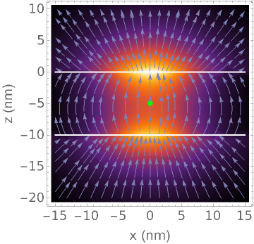
(*MAGNETICFIELDStreamDensityPlot*)xmin=-15;(*Plotlimitsinnm*)xmax=15;zmin=-20;zmax=10;StreamDensityPlot[BfieldnmmT[x,z],{x,xmin,xmax},{z,zmin,zmax},FrameTrue,FrameLabel{"x (nm)","z (nm)"},LabelStyleDirective[FontFamily"Helvetica",18],StreamScale{0.1,Automatic,0.025},StreamStyleDirective[Thickness[0.004],RGBColor[0.5,0.5,0.7],AntialiasingTrue],ColorFunctionColorData["SunsetColors"],AspectRatioAutomatic,Epilog{Thick,White,Line[{{xmin,0},{xmax,0}}],Line[{{xmin,-ww*ban*10^9},{xmax,-ww*ban*10^9}}],PointSize[0.025],Green,Point[{{0,lq0*zz0*ban*10^9}}]}]
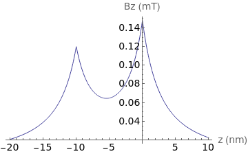
(*Cross-sectionofBzalongthezaxis*)zmin=-20;(*Plotlimitsinnm*)zmax=10;Plot[teslaG*1000*Bfield[0*10^-9/ban,z*10^-9/ban][[2]],{z,zmin,zmax},PlotRangeAll,AxesLabel{"z (nm)","Bz (mT)"},LabelStyleDirective[FontFamily"Helvetica",14]]
Cite this as: Jose L. Movilla, Juan I. Climente, Josep Planelles, "Implementation of a generalized method of image dyons for quasi-two dimensional slabs with ordinary - topological insulator interfaces" from the Notebook Archive (2023), https://notebookarchive.org/2023-02-45ox0tv
Download
