An Extended Goodwin Model with Endogenous Technical Change: Theory and Simulation for the US Economy (1960-2019)
Author
John Cajas Guijarro
Title
An Extended Goodwin Model with Endogenous Technical Change: Theory and Simulation for the US Economy (1960-2019)
Description
Mathematical supplement to accompany Cajas Guijarro (2023): https://mpra.ub.uni-muenchen.de/118878/
Category
Academic Articles & Supplements
Keywords
Extended Goodwin Model, Endogenous Technical Change
URL
http://www.notebookarchive.org/2023-10-cgjt23r/
DOI
https://notebookarchive.org/2023-10-cgjt23r
Date Added
2023-10-27
Date Last Modified
2023-10-27
File Size
1.57 megabytes
Supplements
Rights
CC BY-NC-SA 4.0

Mathematical supplement to accompany Cajas Guijarro (2023): https://mpra.ub.uni-muenchen.de/118878/
An Extended Goodwin Model with Endogenous Technical Change: Theory and Simulation for the US Economy (1960-2019)
An Extended Goodwin Model with Endogenous Technical Change: Theory and Simulation for the US Economy (1960-2019)
John Cajas Guijarro
This notebook extends the two-dimensional Goodwin model of distributive cycles by incorporating endogenous technical change, inspired on some insights originally formulated by Marx. We introduce a three-dimensional dynamical system, expanding the model to include wage share, employment rate, and capital-output ratio as state variables. Theoretical analysis demonstrates an economically meaningful and locally stable equilibrium point, and the Hopf bifurcation theorem reveals the emergence of stable limit cycles as the mechanization-productivity elasticity surpasses a critical value. Econometric estimation of model parameters using ARDL bounds cointegration tests is performed for the US economy from 1965 to 2019. Simulations show damped oscillations, limit cycles, and unstable oscillations, contributing to the understanding of complex capitalist dynamics.
In[]:=
ClearAll["Global`*"]
Parameters estimated for the US economy
In[]:=
simulationUS={δ0.05198494,s0.5626761,β0.01399579,α00.0120001,α10.3334868,ψ00.2678959,ψ10.4210462,γ0.2677537,ρ0.3065009};
The Goodwin Model with a General Capital Accumulation Rate
In[]:=
eq[1]=u[t]w[t]*l[t]/q[t];eq[2]=s(1-u[t])*q[t]k'[t]+δ*k[t];eq[3]=σ[t]k[t]/q[t];eq[4]=k'[t]/k[t]q'[t]/q[t];eq[5]=a[t]q[t]/l[t];eq[6]=a'[t]/a[t]q'[t]/q[t]-l'[t]/l[t];eq[7]=a'[t]/a[t]α;eq[8]=v[t]l[t]/n[t];eq[9]=v'[t]/v[t]l'[t]/l[t]-n'[t]/n[t];eq[10]=n'[t]/n[t]β;eq[11]=(Solve[eq[2],k'[t]][[1,1]]//FullSimplify)/.{RuleEqual};eq[12]=(Solve[{eq[3],eq[4],eq[11]},{q'[t],k'[t],k[t]}][[1,1]]//FullSimplify)/.{RuleEqual};eq[13]=(Solve[{eq[12],eq[6]},{l'[t],q'[t]}][[1,1]]//FullSimplify)/.{RuleEqual};eq[14]=(Solve[{eq[9],eq[13]},{v'[t],l'[t]}][[1,1]]//FullSimplify)/.{RuleEqual};eq[15]=(Solve[{eq[7],eq[10],eq[14]},{v'[t],a'[t],n'[t]}][[1,1]]//FullSimplify)/.{RuleEqual};eq[17]=w'[t]/w[t]-γ+ρ*v[t];eq[18]=u'[t]/u[t]w'[t]/w[t]+l'[t]/l[t]-q'[t]/q[t];eq[19]=(Solve[{eq[18],eq[6]},{u'[t],q'[t]}][[1,1]]//FullSimplify)/.{RuleEqual};eq[20]=(Solve[{eq[17],eq[19]},{u'[t],w'[t]}][[1,1]]//FullSimplify)/.{RuleEqual};eq[21]=(Solve[{eq[7],eq[20]},{u'[t],a'[t]}][[1,1]]//FullSimplify)/.{RuleEqual};
An Extended Goodwin Model with Endogenous Technical Change
In[]:=
eq[23]=m[t]k[t]/l[t];eq[24]=a'[t]/a[t]α0+α1*(m'[t]/m[t]);eq[25]=σ[t]m[t]/a[t];eq[26]=σ'[t]/σ[t]m'[t]/m[t]-a'[t]/a[t];eq[27]=m'[t]/m[t]-ψ0+ψ1*u[t];eq[28]=(Solve[{eq[24],eq[27]},{a'[t],m'[t]}][[1,1]]//FullSimplify)/.{RuleEqual};eq[29]=(Solve[{eq[26],eq[27],eq[28]},{σ'[t],m'[t],a'[t]}][[1,1]]//FullSimplify)/.{RuleEqual};eq[30]=σ'[t]/σ[t]k'[t]/k[t]-q'[t]/q[t];eq[31]=(Solve[{eq[3],eq[11],eq[30]},{q'[t],k'[t],k[t]}][[1,1]]//FullSimplify)/.{RuleEqual};eq[32]=(Solve[{eq[6],eq[31]},{l'[t],q'[t]}][[1,1]]//FullSimplify)/.{RuleEqual};eq[33]=(Solve[{eq[9],eq[26],eq[32]},{v'[t],l'[t],σ'[t]}][[1,1]]//FullSimplify)/.{RuleEqual};eq[34]=(Solve[{eq[10],eq[27],eq[33]},{v'[t],m'[t],n'[t]}][[1,1]]//FullSimplify)/.{RuleEqual};eq[35]=(Solve[{eq[17],eq[19],eq[28]},{u'[t],w'[t],a'[t]}][[1,1]]//FullSimplify)/.{RuleEqual};
In[]:=
dynsystem=(Solve[{eq[29],eq[34],eq[35]},{u'[t],v'[t],σ'[t]}][[1]]//FullSimplify)/.{RuleEqual}
Out[]=
[t]-u[t](α0+γ-α1ψ0+α1ψ1u[t]-ρv[t]),[t],[t]-(α0+ψ0-α1ψ0+(-1+α1)ψ1u[t])σ[t]
′
u
′
v
v[t](s-su[t]-(β+δ-ψ0+ψ1u[t])σ[t])
σ[t]
′
σ
In[]:=
dyneq=(Solve[dynsystem/.{u'[t]0,v'[t]0,σ'[t]0},{u[t],v[t],σ[t]}][[1]]//FullSimplify)/.{RuleEqual}
Out[]=
u[t],v[t],σ[t]-
-+ψ0
α0
-1+α1
ψ1
-+γ
α0
-1+α1
ρ
s(α0+ψ0-α1ψ0+(-1+α1)ψ1)
(α0-(-1+α1)(β+δ))ψ1
In[]:=
ZZ=Solve[{Z11-α1,Z2α0+(1-α1)ψ0,Z3γ(1-α1)+α0,Z4ψ1((1-α1)(β+δ)+α0),Z5s((1-α1)(ψ1-ψ0)-α0)},{α1,β,γ,α0,s}][[1]]//FullSimplify
Out[]=
α11-Z1,β-δ+ψ0+,γ,α0Z2-Z1ψ0,s
Z4-Z2ψ1
Z1ψ1
-Z2+Z3+Z1ψ0
Z1
Z5
-Z2+Z1ψ1
In[]:=
ZZR=Solve[{Z11-α1,Z2α0+(1-α1)ψ0,Z3γ(1-α1)+α0,Z4ψ1((1-α1)(β+δ)+α0),Z5s((1-α1)(ψ1-ψ0)-α0)},{Z1,Z2,Z3,Z4,Z5}][[1]]//FullSimplify
Out[]=
{Z11-α1,Z2α0+ψ0-α1ψ0,Z3α0+γ-α1γ,Z4(α0-(-1+α1)(β+δ))ψ1,Z5-sα0+s(-1+α1)(ψ0-ψ1)}
In[]:=
(dyneq/.ZZ)//FullSimplify
Out[]=
u[t],v[t],σ[t]
Z2
Z1ψ1
Z3
Z1ρ
Z5
Z4
Dynamic Analysis of the Extended Model
In[]:=
jacobian=D[{dynsystem[[1,2]],dynsystem[[2,2]],dynsystem[[3,2]]},{{u[t],v[t],σ[t]}}]//FullSimplify
Out[]=
{-α0-γ+α1ψ0-2α1ψ1u[t]+ρv[t],ρu[t],0},-,,,{-(-1+α1)ψ1σ[t],0,-α0+(-1+α1)ψ0+(ψ1-α1ψ1)u[t]}
v[t](s+ψ1σ[t])
σ[t]
s-su[t]-(β+δ-ψ0+ψ1u[t])σ[t]
σ[t]
s(-1+u[t])v[t]
2
σ[t]
In[]:=
jacobianeq=(jacobian/.(dyneq/.{EqualRule}))//FullSimplify
Out[]=
-α1ψ0,,0,,0,,,0,0
α0α1
-1+α1
ρ-+ψ0
α0
-1+α1
ψ1
(α0+γ-α1γ)ψ1(β+δ-ψ0+ψ1)
ρ(α0+ψ0-α1ψ0+(-1+α1)ψ1)
(α0+γ-α1γ)ψ1
2
(α0-(-1+α1)(β+δ))
sρ(α0+ψ0-α1ψ0+(-1+α1)ψ1)
2
(-1+α1)
s(-1+α1)(α0+ψ0-α1ψ0+(-1+α1)ψ1)
α0-(-1+α1)(β+δ)
In[]:=
jacobianeq//MatrixForm
Out[]//MatrixForm=
α0α1 -1+α1 | ρ- α0 -1+α1 ψ1 | 0 |
(α0+γ-α1γ)ψ1(β+δ-ψ0+ψ1) ρ(α0+ψ0-α1ψ0+(-1+α1)ψ1) | 0 | (α0+γ-α1γ) 2 (α0-(-1+α1)(β+δ)) s 2 (-1+α1) |
s(-1+α1)(α0+ψ0-α1ψ0+(-1+α1)ψ1) α0-(-1+α1)(β+δ) | 0 | 0 |
In[]:=
jacobianeqZZ=((jacobianeq/.ZZ)//FullSimplify)
Out[]=
,,0,,0,-Z5ρψ1,,0,0
(-1+Z1)Z2
Z1
Z2ρ
Z1ψ1
Z3(Z4+ψ1(-Z2+Z1ψ1))
Z1ρ(Z2-Z1ψ1)
Z3
2
Z4
2
Z1
Z1Z5ψ1
Z4
In[]:=
jacobianeqZZ//MatrixForm
Out[]//MatrixForm=
(-1+Z1)Z2 Z1 | Z2ρ Z1ψ1 | 0 |
Z3(Z4+ψ1(-Z2+Z1ψ1)) Z1ρ(Z2-Z1ψ1) | 0 | - Z3 2 Z4 2 Z1 |
Z1Z5ψ1 Z4 | 0 | 0 |
In[]:=
ecb1=b1(-Tr[jacobianeq]//FullSimplify)
Out[]=
b1α1-+ψ0
α0
-1+α1
In[]:=
ecb1ZZ=b1((ecb1[[2]]/.ZZ)//FullSimplify)
Out[]=
b1-1+Z2
1
Z1
In[]:=
ecb2=b2(Tr[Minors[jacobianeq]]//FullSimplify)
Out[]=
b2-
(α0+γ-α1γ)-+ψ0(β+δ-ψ0+ψ1)
α0
-1+α1
α0+ψ0-α1ψ0+(-1+α1)ψ1
In[]:=
ecb2ZZ=b2Collect[((ecb2[[2]]/.ZZ[[1;;5]])//FullSimplify),ϕ]
Out[]=
b2
Z2Z31+
Z4
ψ1(-Z2+Z1ψ1)
2
Z1
In[]:=
(*Manualverificationofb2*)(((Z2(Z3Z4(sZ4+ψ1Z5))/(ψ1Z1^2Z4Z5))/.ZZR)-ecb2[[2]])//FullSimplify
Out[]=
0
In[]:=
ecb3=b3(-Det[jacobianeq]//FullSimplify)
Out[]=
b3
(α0+γ-α1γ)(α0-(-1+α1)(β+δ))(α0+ψ0-α1ψ0)
2
(-1+α1)
In[]:=
ecb3ZZ=b3((ecb3[[2]]/.ZZ)//FullSimplify)
Out[]=
b3ψ1
Z2Z3Z4
2
Z1
In[]:=
ecb123=b1*b2-b3((ecb1[[2]]*ecb2[[2]]-ecb3[[2]])//FullSimplify)
Out[]=
b1b2-b3(α0+γ-α1γ)--
(α0-(-1+α1)(β+δ))(α0+ψ0-α1ψ0)
2
(-1+α1)
α1(β+δ-ψ0+ψ1)
2
-+ψ0
α0
-1+α1
α0+ψ0-α1ψ0+(-1+α1)ψ1
In[]:=
{ecb1,ecb2,ecb3,ecb123}/.simulationUS
Out[]=
{b10.0953439,b20.132469,b30.00457323,b1b2-b30.00805686}
In[]:=
ecb123ZZ=b1*b2-b3((ecb123[[2]]/.ZZ)//FullSimplify)
Out[]=
b1b2-b3ψ1(-Z2+Z1ψ1)
Z2Z3((-1+Z1)ψ1-Z4ψ1+Z2(Z4-(-1+Z1)Z1))
2
Z2
2
Z1
2
ψ1
3
Z1
In[]:=
ecb123null=Solve[ecb123[[2]]0,α1]//FullSimplify
Out[]=
α1,α1,α1ψ0(2α0+β+δ+ψ0)-(2(α0+β+δ)+ψ0)ψ1+ψ0(2α0+β+δ+ψ0)-(2(α0+β+δ)+ψ0)ψ1-
α0+γ
γ
α0+ψ0
ψ0
1
2-2(β+δ+ψ0)ψ1
2
ψ0
β+δ-ψ0+ψ1
(β+δ-ψ0)+(4α0(α0+β+δ)+)ψ1
,α12
ψ0
2
ψ0
1
2-2(β+δ+ψ0)ψ1
2
ψ0
β+δ-ψ0+ψ1
(β+δ-ψ0)+(4α0(α0+β+δ)+)ψ1
2
ψ0
2
ψ0
In[]:=
(*Wechoosethethirdroot*)ecb123null/.simulationUS
Out[]=
{{0.3334871.04482},{0.3334871.04479},{0.3334870.1527},{0.3334871.04757}}
In[]:=
paramHB=α1c(ecb123null[[3,1,2]]//FullSimplify)
Out[]=
α1cψ0(2α0+β+δ+ψ0)-(2(α0+β+δ)+ψ0)ψ1+
1
2-2(β+δ+ψ0)ψ1
2
ψ0
β+δ-ψ0+ψ1
(β+δ-ψ0)+(4α0(α0+β+δ)+)ψ1
2
ψ0
2
ψ0
In[]:=
(*Manualverificationofα1c*)Z6=(α0+β+δ)ψ1+(α0+β+δ+ψ0)(ψ1-ψ0)-α0ψ0;Z7=(β+δ+ψ1-ψ0)((β+δ+ψ1-ψ0)ψ0^2+4α0ψ1(α0+β+δ));Z8=(β+δ)ψ1+ψ0(ψ1-ψ0);solα1=α1c((Z6-Z7^(1/2))/(2Z8))(paramHB[[2]]-solα1[[2]])/.simulationUS
Out[]=
α1c-α0ψ0+(α0+β+δ)ψ1+(α0+β+δ+ψ0)(-ψ0+ψ1)-
(β+δ-ψ0+ψ1)(4α0(α0+β+δ)ψ1+(β+δ-ψ0+ψ1))
(2((β+δ)ψ1+ψ0(-ψ0+ψ1)))2
ψ0
Out[]=
2.77556×
-17
10
In[]:=
dydα1=D[ecb123[[2]],α1]//FullSimplify(dydα1/.{α1paramHB[[2]]})/.simulationUS
Out[]=
γ(α0-(-1+α1)(β+δ))(α0+ψ0-α1ψ0)
2
(-1+α1)
α1γ(β+δ-ψ0+ψ1)
2
-+ψ0
α0
-1+α1
α0+ψ0-α1ψ0+(-1+α1)ψ1
(α0-(-1+α1)(β+δ))ψ0
2
(-1+α1)
(β+δ)(α0+ψ0-α1ψ0)
2
(-1+α1)
2(α0-(-1+α1)(β+δ))(α0+ψ0-α1ψ0)
3
(-1+α1)
α1(-ψ0+ψ1)(β+δ-ψ0+ψ1)
2
-+ψ0
α0
-1+α1
2
(α0+ψ0-α1ψ0+(-1+α1)ψ1)
2
-+ψ0
α0
-1+α1
α0+ψ0-α1ψ0+(-1+α1)ψ1
2α0α1(α0+ψ0-α1ψ0)(β+δ-ψ0+ψ1)
3
(-1+α1)
Out[]=
0.0415772
Simulating the Extended Goodwin Model for the US Economy
In[]:=
(*Estimatedequilibrium*)dyneqUS=dyneq/.simulationUS
Out[]=
{u[t]0.679023,v[t]0.932324,σ[t]2.15045}
In[]:=
ZZR/.simulationUS
Out[]=
{Z10.666513,Z20.190556,Z30.190461,Z40.023569,Z50.0506839}
In[]:=
{Z6,Z7,Z8}/.simulationUS
Out[]=
{0.0825899,0.00379155,0.0688093}
(*Stabilityconditions*)
In[]:=
{0<α0<1,paramHB[[2]]<α1<1,ψ0<ψ1,α0<(1-α1)(ψ1-ψ0)}/.simulationUS
Out[]=
{True,True,True,True}
In[]:=
paramHB/.simulationUS
Out[]=
α1c0.1527
(*USdata:wageshareu*)
In[]:=
dataUSu={0.68163977429261`,0.6762079686932578`,0.6703020187888448`,0.6672112079658565`,0.6637166837270754`,0.6551652655601355`,0.6540088798912439`,0.6624361375639994`,0.6667170912992468`,0.6786538315462496`,0.6872798811799025`,0.6768584519584151`,0.6747308610033602`,0.6711950252797722`,0.6769697061039261`,0.6622405996129658`,0.6557701637474288`,0.6547657963622824`,0.6518295348257737`,0.6524805477480169`,0.6611751201971099`,0.6531424787125644`,0.6614561642360852`,0.6474789638475258`,0.6405654088484588`,0.6402262537412091`,0.6446686006904069`,0.6515306293740686`,0.6548645509206995`,0.6469221146649571`,0.6516900617840478`,0.6559207015052103`,0.6562631796482513`,0.6500498808399241`,0.6429132529781422`,0.6402874484434816`,0.6362012734420653`,0.6371885470875576`,0.6471446668881708`,0.6461861791886708`,0.656133893474094`,0.6550992427393026`,0.6458015541522647`,0.6398076159505142`,0.6355251510171781`,0.6260167549115426`,0.6257361125400861`,0.6274695847761869`,0.6274878326745569`,0.6166215991573578`,0.6055576917548396`,0.604905663258957`,0.6038348356847936`,0.6003008360365397`,0.6025444916173803`,0.6086108325907355`,0.6088389974256897`,0.6106143857603832`,0.6095261014040809`,0.6105119147514427`};
(*USdata:employmentratev*)
In[]:=
dataUSv={0.9500438922858623`,0.9390440921094333`,0.9500795783011609`,0.9475348278448863`,0.9522694931492633`,0.9588684157082397`,0.9657805564671591`,0.9658792221741144`,0.9677726015726336`,0.9686573146647224`,0.9557590714197094`,0.9464285601197217`,0.9488737507995864`,0.955182333972687`,0.9486598495815116`,0.9218222745633425`,0.9290841260576144`,0.9345362937509049`,0.9437204277625205`,0.9464446225216421`,0.934374808465304`,0.9297567762328705`,0.9102749732419412`,0.9111955646982628`,0.9306971972336341`,0.9336784183317703`,0.9355999749717907`,0.9429481737522166`,0.9492666309776345`,0.9514866629395725`,0.948336726684943`,0.9369104577321784`,0.9305489138443996`,0.9358688140494529`,0.943395332820968`,0.9480561647279049`,0.9498170430365321`,0.9540492150158328`,0.9580728357886493`,0.9608915138575733`,0.9628343083994986`,0.9557819590913228`,0.9456612682496546`,0.9432265244849364`,0.9475709166243108`,0.9515880102040817`,0.955897267911026`,0.9557881981098486`,0.9444205701188941`,0.9106606474951712`,0.9068909771272167`,0.9137847560180214`,0.9222866574363844`,0.9292477409508381`,0.9409066664044776`,0.9495476418814839`,0.9533325305557228`,0.9582301645177443`,0.9626831224449148`,0.9648807586870463`};
(*USdata:capital/outputratiosigmaσ*)
In[]:=
dataUSs={3.260911137629554`,3.254930972075523`,3.146045466649613`,3.100644627336144`,3.019220530160392`,2.92333055189236`,2.821961574882685`,2.837466443866576`,2.797110607773657`,2.800255309246566`,2.877467022240052`,2.862512258137597`,2.789192293054545`,2.720296417704668`,2.805461630650369`,2.861047940521664`,2.767238011757639`,2.707796479468761`,2.631926152765534`,2.622036332443594`,2.700016552879566`,2.706963656661053`,2.800988423354921`,2.732056442146635`,2.619976755573849`,2.5898846202387`,2.574209370568309`,2.557260041107037`,2.520847364815606`,2.494142446044449`,2.507068480589243`,2.562973683593347`,2.522234867594404`,2.501491563464673`,2.466157408343646`,2.454625656293911`,2.427332388390513`,2.392154654671856`,2.363679941574662`,2.334589788138811`,2.323762053245685`,2.371516757680217`,2.401822932631213`,2.404990925244657`,2.392627320994428`,2.392081723913996`,2.406604395688412`,2.426136397804594`,2.475860092616186`,2.56530800727826`,2.52333456173537`,2.515255098503582`,2.49663241700221`,2.494071561016768`,2.484840680499102`,2.465863076111207`,2.472800286315461`,2.469508606426756`,2.455340481354787`,2.453816908435104`};
(*Identifyinginitialconditions*)
In[]:=
distance=List[];
In[]:=
Do[initialcondS1={u[1]dataUSu[[i]],v[1]dataUSv[[i]],σ[1]dataUSs[[i]]};S1=NDSolve[Join[dynsystem,initialcondS1]/.simulationUS,{u,v,σ},{t,1,60}];AppendTo[distance,Mean[Table[((dataUSu[[x]]-S1[[1,1,2]][x])^2+(dataUSv[[x]]-S1[[1,2,2]][x])^2+(dataUSs[[x]]-S1[[1,3,2]][x])^2)^0.5,{x,1,60}]]];,{i,1,60}]
In[]:=
min=Position[distance,Min[distance]][[1,1]]
Out[]=
3
(*SimulationfortheUSeconomy*)
In[]:=
initialcondS1={u[1]dataUSu[[min]],v[1]dataUSv[[min]],σ[1]dataUSs[[min]]}
Out[]=
{u[1]0.670302,v[1]0.95008,σ[1]3.14605}
In[]:=
S1=NDSolve[Join[dynsystem,initialcondS1]/.simulationUS,{u,v,σ},{t,1,1000}];
(*Figure1*)
In[]:=
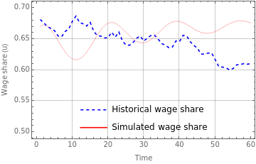
fig1a=Legended[Show[ListLinePlot[dataUSu,PlotStyle{Dashed,Blue}],Plot[S1[[1,1,2]][t],{t,1,60},PlotStyle{Red,Thickness[0.001]}],PlotRange{0.5,0.7},AxesOrigin{0,0.5},FrameLabel{"Time","Wage share (u)"},FrameTrue,GridLinesAutomatic],Placed[LineLegend[{{Dashed,Blue},Red},{"Historical wage share","Simulated wage share"}],{0.5,0.15}]]
Out[]=
In[]:=
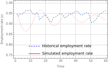
fig1b=Legended[Show[ListLinePlot[dataUSv,PlotStyleDashed],Plot[S1[[1,2,2]][t],{t,1,60},PlotStyle{Red,Thickness[0.001]}],PlotRange{0.75,1},AxesOrigin{0,0.75},FrameLabel{"Time","Employment rate (v)"},FrameTrue,GridLinesAutomatic],Placed[LineLegend[{{Dashed,Blue},Red},{"Historical employment rate","Simulated employment rate"}],{0.5,0.15}]]
Out[]=
In[]:=
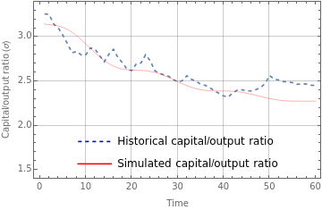
fig1c=Legended[Show[ListLinePlot[dataUSs,PlotStyleDashed],Plot[S1[[1,3,2]][t],{t,1,60},PlotStyle{Red,Thickness[0.001]}],PlotRange{1.5,3.3},AxesOrigin{0,1.5},FrameLabel{"Time","Capital/output ratio (σ)"},FrameTrue,GridLinesAutomatic],Placed[LineLegend[{{Dashed,Blue},Red},{"Historical capital/output ratio","Simulated capital/output ratio"}],{0.5,0.15}]]
Out[]=
In[]:=
(*Figure2*)
In[]:=
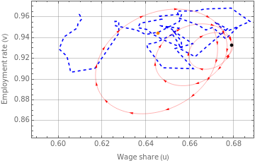
fig2a=Legended[Show[ListLinePlot[Transpose@{dataUSu,dataUSv},PlotStyle{Blue,Dashed}],ParametricPlot[{S1[[1,1,2]][t],S1[[1,2,2]][t]},{t,1,60},PlotStyle{Red,Thickness[0.001]}]/.Line[x_]{Arrowheads[Flatten[{0,ConstantArray[0.018,30]}]],Arrow[x]},Graphics[{PointSize[0.015],Black,Point[{dyneqUS[[1,2]],dyneqUS[[2,2]]}]}],Graphics[{PointSize[0.015],Orange,Point[{averageUS[[1,2]],averageUS[[2,2]]}]}],PlotRangeAll,AxesOrigin{0.59,0.85},FrameLabel{"Wage share (u)","Employment rate (v)"},FrameTrue,GridLinesAutomatic],LineLegend[{{Dashed,Blue},Orange,Red,Black},{"Historical trajectory","Historical average","Simulated trajectory","Simulated equilibrium"}]]
Out[]=
 |
|
In[]:=
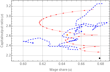
fig2b=Legended[Show[ListLinePlot[Transpose@{dataUSu,dataUSs},PlotStyle{Blue,Dashed}],ParametricPlot[{S1[[1,1,2]][t],S1[[1,3,2]][t]},{t,1,60},PlotStyle{Red,Thickness[0.001]}]/.Line[x_]{Arrowheads[Flatten[{0,ConstantArray[0.018,30]}]],Arrow[x]},Graphics[{PointSize[0.015],Black,Point[{dyneqUS[[1,2]],dyneqUS[[3,2]]}]}],Graphics[{PointSize[0.015],Orange,Point[{averageUS[[1,2]],averageUS[[3,2]]}]}],PlotRangeAll,AxesOrigin{0.59,2.2},FrameLabel{"Wage share (u)","Capital/output ratio (σ)"},FrameTrue,GridLinesAutomatic],LineLegend[{{Dashed,Blue},Orange,Red,Black},{"Historical trajectory","Historical average","Simulated trajectory","Simulated equilibrium"}]]
Out[]=
 |
|
In[]:=
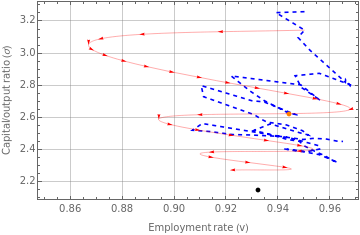
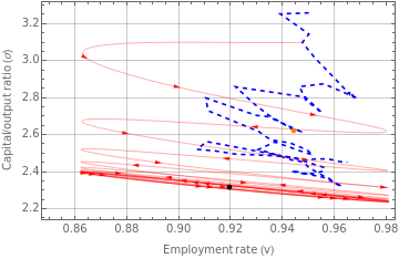
fig2c=Legended[Show[ListLinePlot[Transpose@{dataUSv,dataUSs},PlotStyle{Blue,Dashed}],ParametricPlot[{S1[[1,2,2]][t],S1[[1,3,2]][t]},{t,1,60},PlotStyle{Red,Thickness[0.001]}]/.Line[x_]{Arrowheads[Flatten[{0,ConstantArray[0.017,30]}]],Arrow[x]},Graphics[{PointSize[0.015],Black,Point[{dyneqUS[[2,2]],dyneqUS[[3,2]]}]}],Graphics[{PointSize[0.015],Orange,Point[{averageUS[[2,2]],averageUS[[3,2]]}]}],PlotRangeAll,AxesOrigin{0.85,2.2},FrameLabel{"Employment rate (v)","Capital/output ratio (σ)"},FrameTrue,GridLinesAutomatic],LineLegend[{{Dashed,Blue},Orange,Red,Black},{"Historical trajectory","Historical average","Simulated trajectory","Simulated equilibrium"}]]
Out[]=
 |
|
(*Figure3*)
In[]:=
fig3=Legended[Show[ListPointPlot3D[Transpose@{dataUSu,dataUSv,dataUSs},PlotStyle{Blue,PointSize[0.013]}],ParametricPlot3D[{S1[[1,1,2]][t],S1[[1,2,2]][t],S1[[1,3,2]][t]},{t,1,60},PlotStyle{Red,Thickness[0.001]}]/.Line[x_]{Arrowheads[Flatten[{0,ConstantArray[0.003,8]}]],Arrow[x]},Graphics3D[{PointSize[0.015],Black,Point[{dyneqUS[[1,2]],dyneqUS[[2,2]],dyneqUS[[3,2]]}]}],Graphics3D[{PointSize[0.015],Orange,Point[{averageUS[[1,2]],averageUS[[2,2]],averageUS[[3,2]]}]}],PlotRangeAll,AxesStyleGrayLevel[0.5],BoxStyleGrayLevel[0.8],AxesLabel{"u","v","σ"}],LineLegend[{{Dashed,Blue},Orange,Red,Black},{"Historical data","Historical average","Simulated trajectory","Simulated equilibrium"}]]
Out[]=
 |
|
In[]:=
(*Historicalmean*)averageUS={u[t]Mean[dataUSu],v[t]Mean[dataUSv],σ[t]Mean[dataUSs]}
Out[]=
{u[t]0.64545,v[t]0.944448,σ[t]2.62379}
(*Relativedifferencebewteenhistoricalmeanandequilibrium*)Table[(dyneqUS[[x,2]]/averageUS[[x,2]]-1)*100,{x,1,3}]
Out[]=
{5.20154,-1.28378,-18.0403}
(*MSEasaproportionofthehistoricalmean*)
In[]:=
{((Mean[Table[(dataUSu[[x]]-S1[[1,1,2]][x])^2,{x,1,60}]])^0.5)/Mean[dataUSu]*100,((Mean[Table[(dataUSv[[x]]-S1[[1,2,2]][x])^2,{x,1,60}]])^0.5)/Mean[dataUSv]*100,((Mean[Table[(dataUSs[[x]]-S1[[1,3,2]][x])^2,{x,1,60}]])^0.5)/Mean[dataUSs]*100}
Out[]=
{5.93433,4.13404,4.6355}
Limit Cycles and the Mechanization-Productivity Relationship
(*Simulationoflimitcycles*)
In[]:=
simulationLC=simulationUS;simulationLC[[5]]=α1(paramHB[[2]]/.simulationUS);simulationLC
Out[]=
{δ0.0519849,s0.562676,β0.0139958,α00.0120001,α10.1527,ψ00.267896,ψ10.421046,γ0.267754,ρ0.306501}
(*DynamicequilibriumLC*)
In[]:=
dyneqLC=dyneq/.simulationLC
Out[]=
{u[t]0.6699,v[t]0.91979,σ[t]2.31759}
(*Identifyinginitialconditions*)
In[]:=
distance=List[];
In[]:=
Do[initialcondS2={u[1]dataUSu[[i]],v[1]dataUSv[[i]],σ[1]dataUSs[[i]]};S2=NDSolve[Join[dynsystem,initialcondS2]/.simulationLC,{u,v,σ},{t,1,60}];AppendTo[distance,Mean[Table[((dataUSu[[x]]-S2[[1,1,2]][x])^2+(dataUSv[[x]]-S2[[1,2,2]][x])^2+(dataUSs[[x]]-S2[[1,3,2]][x])^2)^0.5,{x,1,60}]]];,{i,1,60}]
In[]:=
min=Position[distance,Min[distance]][[1,1]]
Out[]=
4
In[]:=
initialcondS2={u[1]dataUSu[[min]],v[1]dataUSv[[min]],σ[1]dataUSs[[min]]}
Out[]=
{u[1]0.667211,v[1]0.947535,σ[1]3.10064}
In[]:=
S2=NDSolve[Join[dynsystem,initialcondS2]/.simulationLC,{u,v,σ},{t,1,1000}]
Out[]=
uInterpolatingFunction
,vInterpolatingFunction
,σInterpolatingFunction
 |
|
|
|
|
|
(*Figure4*)
In[]:=
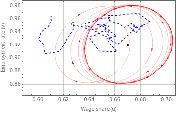
fig4a=Legended[Show[ListLinePlot[Transpose@{dataUSu,dataUSv},PlotStyle{Blue,Dashed}],ParametricPlot[{S2[[1,1,2]][t],S2[[1,2,2]][t]},{t,1,200},PlotStyle{Red,Thickness[0.001]}]/.Line[x_]{Arrowheads[Flatten[{0,ConstantArray[0.02,30]}]],Arrow[x]},Graphics[{PointSize[0.015],Black,Point[{dyneqLC[[1,2]],dyneqLC[[2,2]]}]}],Graphics[{PointSize[0.015],Orange,Point[{averageUS[[1,2]],averageUS[[2,2]]}]}],PlotRangeAll,AxesOrigin{0.59,0.85},FrameLabel{"Wage share (u)","Employment rate (v)"},FrameTrue,GridLinesAutomatic],LineLegend[{{Dashed,Blue},Orange,Red,Black},{"Historical trajectory","Historical average","Simulated trajectory","Simulated equilibrium"}]]
Out[]=
 |
|
In[]:=
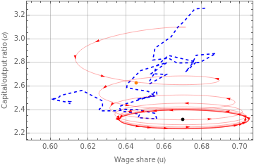
fig4b=Legended[Show[ListLinePlot[Transpose@{dataUSu,dataUSs},PlotStyle{Blue,Dashed}],ParametricPlot[{S2[[1,1,2]][t],S2[[1,3,2]][t]},{t,1,200},PlotStyle{Red,Thickness[0.001]}]/.Line[x_]{Arrowheads[Flatten[{0,ConstantArray[0.02,30]}]],Arrow[x]},Graphics[{PointSize[0.015],Black,Point[{dyneqLC[[1,2]],dyneqLC[[3,2]]}]}],Graphics[{PointSize[0.015],Orange,Point[{averageUS[[1,2]],averageUS[[3,2]]}]}],PlotRangeAll,AxesOrigin{0.59,2.2},FrameLabel{"Wage share (u)","Capital/output ratio (σ)"},FrameTrue,GridLinesAutomatic],LineLegend[{{Dashed,Blue},Orange,Red,Black},{"Historical trajectory","Historical average","Simulated trajectory","Simulated equilibrium"}]]
Out[]=
 |
|
In[]:=
fig4c=Legended[Show[ListLinePlot[Transpose@{dataUSv,dataUSs},PlotStyle{Blue,Dashed}],ParametricPlot[{S2[[1,2,2]][t],S2[[1,3,2]][t]},{t,1,200},PlotStyle{Red,Thickness[0.001]}]/.Line[x_]{Arrowheads[Flatten[{0,ConstantArray[0.02,30]}]],Arrow[x]},Graphics[{PointSize[0.015],Black,Point[{dyneqLC[[2,2]],dyneqLC[[3,2]]}]}],Graphics[{PointSize[0.015],Orange,Point[{averageUS[[2,2]],averageUS[[3,2]]}]}],PlotRangeAll,AxesOrigin{0.85,2.2},FrameLabel{"Employment rate (v)","Capital/output ratio (σ)"},FrameTrue,GridLinesAutomatic],LineLegend[{{Dashed,Blue},Orange,Red,Black},{"Historical trajectory","Historical average","Simulated trajectory","Simulated equilibrium"}]]
Out[]=
 |
|
(*Figure5*)
In[]:=
fig5=Legended[Show[ListPointPlot3D[Transpose@{dataUSu,dataUSv,dataUSs},PlotStyle{Blue,PointSize[0.013]}],ParametricPlot3D[{S2[[1,1,2]][t],S2[[1,2,2]][t],S2[[1,3,2]][t]},{t,1,200},PlotStyle{Red,Thickness[0.001]}]/.Line[x_]{Arrowheads[Flatten[{0,ConstantArray[0.005,15]}]],Arrow[x]},Graphics3D[{PointSize[0.015],Black,Point[{dyneqLC[[1,2]],dyneqLC[[2,2]],dyneqLC[[3,2]]}]}],Graphics3D[{PointSize[0.015],Orange,Point[{averageUS[[1,2]],averageUS[[2,2]],averageUS[[3,2]]}]}],PlotRangeAll,AxesStyleGrayLevel[0.5],BoxStyleGrayLevel[0.8],AxesLabel{"u","v","σ"}],LineLegend[{{Dashed,Blue},Orange,Red,Black},{"Historical data","Historical average","Simulated trajectory","Simulated equilibrium"}]]
Out[]=
 |
|
In[]:=
(*Relativedifferencebewteenhistoricalmeanandequilibrium*)Table[(dyneqLC[[x,2]]/averageUS[[x,2]]-1)*100,{x,1,3}]
Out[]=
{3.78798,-2.61086,-11.6703}
(*MSEasaproportionofthehistoricalmean*)
In[]:=
{((Mean[Table[(dataUSu[[x]]-S2[[1,1,2]][x])^2,{x,1,60}]])^0.5)/Mean[dataUSu]*100,((Mean[Table[(dataUSv[[x]]-S2[[1,2,2]][x])^2,{x,1,60}]])^0.5)/Mean[dataUSv]*100,((Mean[Table[(dataUSs[[x]]-S2[[1,3,2]][x])^2,{x,1,60}]])^0.5)/Mean[dataUSs]*100}
Out[]=
{6.63071,5.82881,4.31434}
(*Simulationofunstableoscillations*)
In[]:=
simulationUO=simulationUS;simulationUO[[5]]=α1(paramHB[[2]]/.simulationUS)-0.01;simulationUO
Out[]=
{δ0.0519849,s0.562676,β0.0139958,α00.0120001,α10.1427,ψ00.267896,ψ10.421046,γ0.267754,ρ0.306501}
(*DynamicequilibriumUO*)
In[]:=
dyneqUO=dyneq/.simulationUO
Out[]=
{u[t]0.669507,v[t]0.919251,σ[t]2.32514}
(*Identifyinginitialconditions*)
In[]:=
distance=List[];
In[]:=
Do[initialcondS3={u[1]dataUSu[[i]],v[1]dataUSv[[i]],σ[1]dataUSs[[i]]};S3=NDSolve[Join[dynsystem,initialcondS3]/.simulationUO,{u,v,σ},{t,1,60}];AppendTo[distance,Mean[Table[((dataUSu[[x]]-S3[[1,1,2]][x])^2+(dataUSv[[x]]-S3[[1,2,2]][x])^2+(dataUSs[[x]]-S3[[1,3,2]][x])^2)^0.5,{x,1,60}]]];,{i,1,60}]
In[]:=
min=Position[distance,Min[distance]][[1,1]]
Out[]=
5
In[]:=
initialcondS3={u[1]dataUSu[[min]],v[1]dataUSv[[min]],σ[1]dataUSs[[min]]}
Out[]=
{u[1]0.663717,v[1]0.952269,σ[1]3.01922}
In[]:=
S3=NDSolve[Join[dynsystem,initialcondS3]/.simulationUO,{u,v,σ},{t,1,1000}]
Out[]=
uInterpolatingFunction
,vInterpolatingFunction
,σInterpolatingFunction
|
|
|
|
|
|
(*Figure6*)
In[]:=
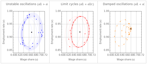
fig6=Show[GraphicsGrid[{{Show[ParametricPlot[{S3[[1,1,2]][t],S3[[1,2,2]][t]},{t,1,200},PlotStyle{Blue,Thickness[0.001]},PlotRange{{0.60,0.72},{0.84,1}},FrameLabel{"Wage share (u)","Employment rate (v)"},FrameTrue,GridLinesAutomatic,PlotLabel"Unstable oscillations (α1 > α1c)"]/.Line[x_]{Arrowheads[Flatten[{0,ConstantArray[0.04,30]}]],Arrow[x]},Graphics[{PointSize[0.03],Black,Point[{dyneqUO[[1,2]],dyneqUO[[2,2]]}]}]],Show[ParametricPlot[{S2[[1,1,2]][t],S2[[1,2,2]][t]},{t,1,200},PlotStyle{Red,Thickness[0.001]},PlotRange{{0.60,0.72},{0.84,1}},FrameLabel{"Wage share (u)","Employment rate (v)"},FrameTrue,GridLinesAutomatic,PlotLabel"Limit cycles (α1 = α1c)"]/.Line[x_]{Arrowheads[Flatten[{0,ConstantArray[0.04,30]}]],Arrow[x]},Graphics[{PointSize[0.03],Black,Point[{dyneqLC[[1,2]],dyneqLC[[2,2]]}]}]],Show[ParametricPlot[{S1[[1,1,2]][t],S1[[1,2,2]][t]},{t,1,200},PlotStyle{Orange,Thickness[0.001]},PlotRange{{0.60,0.72},{0.84,1}},FrameLabel{"Wage share (u)","Employment rate (v)"},FrameTrue,GridLinesAutomatic,PlotLabel"Damped oscillations (α1 < α1c)"]/.Line[x_]{Arrowheads[Flatten[{0,ConstantArray[0.04,30]}]],Arrow[x]},Graphics[{PointSize[0.03],Black,Point[{dyneqUS[[1,2]],dyneqUS[[2,2]]}]}]]}},FrameAll,FrameStyleGrayLevel[0.8]]]
Out[]=
Cite this as: John Cajas Guijarro, "An Extended Goodwin Model with Endogenous Technical Change: Theory and Simulation for the US Economy (1960-2019)" from the Notebook Archive (2023), https://notebookarchive.org/2023-10-cgjt23r
Download
