Debt, Power, and Cycles: A North-South Model of Debt and Distribution (NSDD)
Author
John Cajas Guijarro
Title
Debt, Power, and Cycles: A North-South Model of Debt and Distribution (NSDD)
Description
Mathematical supplement to accompany Cajas Guijarro (2024): "Debt, Power, and Cycles: A North-South Model of Debt and Distribution (NSDD)" (Cuadernos de Economía, in press)
Category
Academic Articles & Supplements
Keywords
North-South model, distributive cycles, foreign debt, stability
URL
http://www.notebookarchive.org/2023-12-cxl4iz7/
DOI
https://notebookarchive.org/2023-12-cxl4iz7
Date Added
2023-12-28
Date Last Modified
2023-12-28
File Size
3.1 megabytes
Supplements
Rights
CC BY-NC-SA 4.0

Mathematical supplement to accompany Cajas Guijarro (2024): “Debt, Power, and Cycles: A North-South Model of Debt and Distribution (NSDD)” (Cuadernos de Economía, in press).
Debt, Power, and Cycles: A North-South Model of Debt and Distribution (NSDD)
Debt, Power, and Cycles: A North-South Model of Debt and Distribution (NSDD)
John Cajas Guijarro
This notebook presents a North-South model of Debt and Distribution (NSDD) that combines the dynamics of the southern foreign debt with the effects of simultaneous distributive cycles coming from both the North and the South. The model includes structural insights from Dutt (1989, 1990), cyclical dynamics from Goodwin (1967), and constraints for the southern balance of payments. This NSDD model studies the stability of the southern foreign debt, and its numerical simulation brings multiple political economy implications. For instance, when the southern debt has a higher interest rate, the distributive cycle deteriorates against southern workers.
(***********************************************************************)(*Limpiamostodo*)ClearAll["Global`*"]
(****************************************Simbologia***************************************)i;(*Subindicedondei=1representaalNorteei=2representaalSur*)Qi[t];(*Produccionnetadelaregioni=1,2*)Li[t];(*Empleoenlaregioni=1,2(medidoenhorasdetrabajoefectivas*)qi[t];(*Productividadlaboralenlaregioni=1,2*)σi;(*Relacioncapital-productovigenteenlaregioni=1,2*)Ki[t];(*Stockdecapital(fijo)delaregioni=1,2*)pi[t];(*Preciodelbienproducidoenlaregioni=1,2*)wi[t];(*Tasadesalariomedioporhoratrabajadaenlaregioni=1,2*)ri[t];(*Tasadegananciaqueobtienenloscapitalistasdelaregioni=1,2desdelaproduccion*)Q1CD[t];(*Demandadomesticadeconsumodelosbienesproducidosenlaregion1*)Q1CF[t];(*Demandaexternadeconsumodelosbienesproducidosenlaregion1*)Q1KD[t];(*Demandadomesticadedeinversiondelosbienesproducidosenlaregion1*)Q1KF[t];(*Demandaexternadeinversiondelosbienesproducidosenlaregion1*)Q2CD[t];(*Demandadomesticadeconsumodelosbienesproducidosenlaregion1*)Q2CF[t];(*Demandaexternadeconsumodelosbienesproducidosenlaregion1*)a;(*FracciondelgastodeconsumoquelasclasessocialesdelNortedestinanabienesextranjeros(delSur)(constante)*)si;(*Tasadeahorrodeloscapitalistasdelaregioni=1,2(constante)*)D2[t];(*StockdedeudaexternaqueelSurmantieneconelNorte*)τ;(*TasadeinteresqueelSurpagaalNorteporsudeudaexterna(constante)*)b;(*FracciondelgastodeconsumoquelasclasessocialesdelSurdestinanabienesextranjeros(delNorte)(constante)*)Ki'[t];(*Acumulaciondecapital(derivadatemporaldelcapitalfijo)delaregioni=1,2*)gi[t];(*Tasadecrecimiento(neto)delcapitaldelaregioni=1,2*)ωi[t];(*Participacionsalarialdelaregioni=1,2(proporciondelproductodelaregionpagadaasustrabajadores)*)Ni[t];(*Ofertadefuerzadetrabajo(poblaciondisponibleparatrabajar)enlaregioni=1,2*)li[t];(*Tasadeempleoenlaregioni=1,2*)p[t];(*PreciorelativodelosbienesdelSurrespectoalosbienesdelNorte,terminosdeintercambiodelSur*)vi[t];(*Salariorealdelostrabajadoresdelaregioni=1,2*)f[t];(*ProporcionentreladeudaexternayelstockdecapitaldelSur*)k[t];(*Composicionregionaldelcapital(ratioentreelstockdecapitaldelNorteydelSur)*)B2[t];(*DeficitcomercialdelSur(igualalsuperavitcomercialdelNorte)medidoenterminosdelbiendelNorte*)π1[t];(*TasadeganancianetadeloscapitalistasdelNorte(tomandoencuentainteresesdedeudaexternadelSur)*)γ0;(*TasadecrecimientoautonomodelcapitaldelNorte(constante)*)γ1;(*Efectodeπ1[t]sobrelatasadecrecimientodelcapitaldelNorte(efectorentabilidad)(constante)*)ρ0i;(*Representaciondelpoderdeloscapitalistasdelaregioni=1,2deempujarelsalariorealalabaja(constante)*)ρli;(*Representaciondelpoderdelostrabajadoresdelaregioni=1,2deempujarelsalariorealalalza(constante)*)αi;(*Tasadecrecimientodelaproductividadlaboraldelaregioni=1,2(constante)*)βi;(*Tasadecrecimientodelapoblaciondisponibleparatrabajardelaregioni=1,2(constante)*)
(************************************************************************)(**********Primeraparte:esquemageneraldeinteraccionesNorte-Sur**********)(************************************************************************)
In[]:=
ec[1]={Q1[t]q1[t]*L1[t],Q2[t]q2[t]*L2[t]};
In[]:=
ec[2]={σ1K1[t]/Q1[t],σ2K2[t]/Q2[t]};
In[]:=
ec[3]={p1[t]*Q1[t]w1[t]*L1[t]+r1[t]*p1[t]*K1[t],p2[t]*Q2[t]w2[t]*L2[t]+r2[t]*p1[t]*K2[t]};
In[]:=
ec[4]=Q1CD[t]+Q1CF[t]+Q1KD[t]+Q1KF[t]-Q1[t]0;
In[]:=
ec[5]=Q2CD[t]+Q2CF[t]-Q2[t]0;
In[]:=
ec[6]=p1[t]*Q1CD[t](1-a)*(w1[t]*L1[t]+(1-s1)*(r1[t]*p1[t]*K1[t]+τ*p1[t]*D2[t]));
In[]:=
ec[7]=p2[t]*Q2CF[t]a*(w1[t]*L1[t]+(1-s1)*(r1[t]*p1[t]*K1[t]+τ*p1[t]*D2[t]));
In[]:=
ec[8]=p2[t]*Q2CD[t](1-b)*(w2[t]*L2[t]+(1-s2)*(r2[t]*p1[t]*K2[t]-τ*p1[t]*D2[t]));
In[]:=
ec[9]=p1[t]*Q1CF[t]b*(w2[t]*L2[t]+(1-s2)*(r2[t]*p1[t]*K2[t]-τ*p1[t]*D2[t]));
In[]:=
ec[10]=Q1KD[t]g1[t]*K1[t];
In[]:=
ec[11]=Q1KF[t]g2[t]*K2[t];
In[]:=
ec[12]={ω1[t](w1[t]*L1[t])/(p1[t]*Q1[t]),ω2[t](w2[t]*L2[t])/(p2[t]*Q2[t])};
In[]:=
ec[13]={l1[t]L1[t]/N1[t],l2[t]L2[t]/N2[t]};
In[]:=
ec[14]=p[t]p2[t]/p1[t];
In[]:=
ec[15]={v1[t](w1[t]/p1[t])*((1-a)+a/p[t]),v2[t](w2[t]/p2[t])*((1-b)+b*p[t])};
In[]:=
ec[16]=f[t]D2[t]/K2[t];
In[]:=
ec[17]=k[t]K1[t]/K2[t];
In[]:=
ec[18]=B2[t](Q1CF[t]+Q1KF[t])-p[t]*Q2CF[t];
In[]:=
simplificacion1={s11,s21,b1};
In[]:=
deduccion1=Solve[{ec[1][[1]],ec[1][[2]],ec[2][[1]],ec[2][[2]],ec[3][[1]],ec[3][[2]],ec[4],ec[5],ec[6],ec[7],ec[8],ec[9],ec[10],ec[11],ec[12][[1]],ec[12][[2]],ec[13][[1]],ec[13][[2]],ec[14],ec[15][[1]],ec[15][[2]],ec[16],ec[17],ec[18]}/.simplificacion1,{L1[t],L2[t],g2[t],p[t],r1[t],r2[t],Q1[t],Q2[t],Q1CD[t],Q2CF[t],Q2CD[t],Q1CF[t],Q1KD[t],Q1KF[t],w1[t],w2[t],v1[t],v2[t],l1[t],l2[t],p2[t],K2[t],K1[t],B2[t]}]//FullSimplify
Out[]=
L1[t],L2[t],g2[t]-,p[t],r1[t],r2[t]-,Q1[t],Q2[t],Q1CD[t]-,Q2CF[t],Q2CD[t]0,Q1CF[t],Q1KD[t],Q1KF[t]-,w1[t]p1[t]q1[t]ω1[t],w2[t],v1[t]q1[t]+ω1[t]-aω1[t],v2[t],l1[t],l2[t],p2[t],K2[t],K1[t],B2[t]-
D2[t]k[t]
σ1f[t]q1[t]
D2[t]
σ2f[t]q2[t]
k[t](-1+σ1g1[t]+ω1[t](1-a+aω2[t]))
σ1
aσ2k[t]ω1[t]
σ1
1-ω1[t]
σ1
ak[t]ω1[t](-1+ω2[t])
σ1
D2[t]k[t]
σ1f[t]
D2[t]
σ2f[t]
(-1+a)D2[t]k[t]ω1[t]
σ1f[t]
D2[t]
σ2f[t]
aD2[t]k[t]ω1[t]ω2[t]
σ1f[t]
D2[t]g1[t]k[t]
f[t]
D2[t]k[t](-1+σ1g1[t]+ω1[t](1-a+aω2[t]))
σ1f[t]
aσ2k[t]p1[t]q2[t]ω1[t]ω2[t]
σ1
σ1
σ2k[t]
aσ2k[t]q2[t]ω1[t]ω2[t]
σ1
D2[t]k[t]
σ1f[t]N1[t]q1[t]
D2[t]
σ2f[t]N2[t]q2[t]
aσ2k[t]p1[t]ω1[t]
σ1
D2[t]
f[t]
D2[t]k[t]
f[t]
D2[t]k[t](-1+σ1g1[t]+ω1[t])
σ1f[t]
In[]:=
ec[19]=deduccion1[[1,3]]/.{RuleEqual}
Out[]=
g2[t]-
k[t](-1+σ1g1[t]+ω1[t](1-a+aω2[t]))
σ1
In[]:=
ec[20]=deduccion1[[1,4]]/.{RuleEqual}
Out[]=
p[t]
aσ2k[t]ω1[t]
σ1
In[]:=
(*************************************************************************)(**********Segundaparte:(in)estabilidaddeladeudaexternadelSur**********)(*************************************************************************)
In[]:=
ec[21]=k'[t]/k[t]g1[t]-g2[t];
In[]:=
ec[22]=π1[t]r1[t]+τ*f[t]/k[t];
In[]:=
ec[23]=g1[t]γ0+γ1*π1[t];
In[]:=
ec[24]=D2'[t]B2[t]+τ*D2[t];
In[]:=
ec[25]=f'[t]/f[t]D2'[t]/D2[t]-g2[t];
In[]:=
simplificacion2=Join[simplificacion1,{γ00}]
Out[]=
{s11,s21,b1,γ00}
In[]:=
deduccion2=Solve[{ec[1][[1]],ec[1][[2]],ec[2][[1]],ec[2][[2]],ec[3][[1]],ec[3][[2]],ec[4],ec[5],ec[6],ec[7],ec[8],ec[9],ec[10],ec[11],ec[12][[1]],ec[12][[2]],ec[13][[1]],ec[13][[2]],ec[14],ec[15][[1]],ec[15][[2]],ec[16],ec[17],ec[18],ec[21],ec[22],ec[23],ec[24],ec[25]}/.simplificacion2,{L1[t],L2[t],g2[t],p[t],r1[t],r2[t],Q1[t],Q2[t],Q1CD[t],Q2CF[t],Q2CD[t],Q1CF[t],Q1KD[t],Q1KF[t],w1[t],w2[t],v1[t],v2[t],l1[t],l2[t],p2[t],K2[t],K1[t],B2[t],k'[t],π1[t],g1[t],D2'[t],f'[t]}]//FullSimplify
Out[]=
L1[t],L2[t],g2[t]-γ1τf[t]+,p[t],r1[t],r2[t]-,Q1[t],Q2[t],Q1CD[t]-,Q2CF[t],Q2CD[t]0,Q1CF[t],Q1KD[t],Q1KF[t]D2[t]-γ1τ+,w1[t]p1[t]q1[t]ω1[t],w2[t],v1[t]q1[t]+ω1[t]-aω1[t],v2[t],l1[t],l2[t],p2[t],K2[t],K1[t],B2[t]D2[t]-γ1τ+,[t]γ1τf[t](1+k[t])+,π1[t]+,g1[t],[t]-,[t](γ1σ1τ+(-1+γ1)k[t](-1+ω1[t])+f[t](-(-1+γ1)σ1τ+k[t](-1+γ1+ω1[t](1-a-γ1+aω2[t]))))
D2[t]k[t]
σ1f[t]q1[t]
D2[t]
σ2f[t]q2[t]
k[t](1-γ1+ω1[t](-1+a+γ1-aω2[t]))
σ1
aσ2k[t]ω1[t]
σ1
1-ω1[t]
σ1
ak[t]ω1[t](-1+ω2[t])
σ1
D2[t]k[t]
σ1f[t]
D2[t]
σ2f[t]
(-1+a)D2[t]k[t]ω1[t]
σ1f[t]
D2[t]
σ2f[t]
aD2[t]k[t]ω1[t]ω2[t]
σ1f[t]
γ1D2[t](σ1τf[t]+k[t]-k[t]ω1[t])
σ1f[t]
k[t](1-γ1+ω1[t](-1+a+γ1-aω2[t]))
σ1f[t]
aσ2k[t]p1[t]q2[t]ω1[t]ω2[t]
σ1
σ1
σ2k[t]
aσ2k[t]q2[t]ω1[t]ω2[t]
σ1
D2[t]k[t]
σ1f[t]N1[t]q1[t]
D2[t]
σ2f[t]N2[t]q2[t]
aσ2k[t]p1[t]ω1[t]
σ1
D2[t]
f[t]
D2[t]k[t]
f[t]
(-1+γ1)k[t](-1+ω1[t])
σ1f[t]
′
k
k[t](γ1-γ1ω1[t]+k[t](-1+γ1+ω1[t](1-a-γ1+aω2[t])))
σ1
τf[t]
k[t]
1-ω1[t]
σ1
γ1(σ1τf[t]+k[t]-k[t]ω1[t])
σ1k[t]
′
D2
(-1+γ1)D2[t](σ1τf[t]+k[t]-k[t]ω1[t])
σ1f[t]
′
f
1
σ1
2
f[t]
In[]:=
(*Sistemadinamico26-27*)
In[]:=
ec[26]=deduccion2[[1,25]]/.{RuleEqual}
Out[]=
′
k
k[t](γ1-γ1ω1[t]+k[t](-1+γ1+ω1[t](1-a-γ1+aω2[t])))
σ1
In[]:=
ec[27]=deduccion2[[1,29]]/.{RuleEqual}
Out[]=
′
f
1
σ1
2
f[t]
In[]:=
(*Obtencionyanalisisdelalineanulak'=0*)
In[]:=
ec[28]=(Solve[ec[26]/.{k'[t]0},f[t]][[1,1]]//FullSimplify)/.{RuleEqual}
Out[]=
f[t]
k[t](γ1(-1+ω1[t])+k[t](1-γ1+ω1[t](-1+a+γ1-aω2[t])))
γ1σ1τ(1+k[t])
In[]:=
ec[29]=(Solve[ec[28]/.{f[t]0},k[t]][[2,1]]//FullSimplify)/.{RuleEqual,k[t]kA[t]}
Out[]=
kA[t]
γ1-γ1ω1[t]
1-γ1+ω1[t](-1+a+γ1-aω2[t])
In[]:=
ec[30]=dfnD[ec[28][[2]],k[t]]//FullSimplify
Out[]=
dfn(γ1(-1+ω1[t])+2k[t](1-γ1+ω1[t](-1+a+γ1-aω2[t]))+(1-γ1+ω1[t](-1+a+γ1-aω2[t])))
1
γ1σ1τ
2
(1+k[t])
2
k[t]
In[]:=
ec[31]=d2fnD[ec[30][[2]],k[t]]//FullSimplify
Out[]=
d2fn
2-2ω1[t](1-a+aω2[t])
γ1σ1τ
3
(1+k[t])
In[]:=
(*Parametrosparasimulacion1*)
In[]:=
paramsim1={a0.8,γ10.8,σ13,σ23,τ0.05,ω1[t]0.5,ω2[t]0.5};
In[]:=
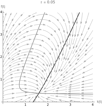
(*Figura1:lineanulak'=0ydinamicadek*)
In[]:=
figura1=Show[ContourPlot[Evaluate[{ec[28]}/.paramsim1],{k[t],0,4},{f[t],0,4},ContourStyleBlack,FrameFalse,AxesTrue,AxesLabel{"Composicion regional del capital k[t]","Endeudamiento relativo del Sur f[t]"}],StreamPlot[{ec[26][[2]]/.paramsim1,0},{k[t],0,4},{f[t],0,4},StreamStyleGrayLevel[0.66],StreamScale0.13]]
Out[]=

In[]:=
(*Obtencionyanalisisdelalineanulaf'=0*)
In[]:=
ec[32]=(Solve[ec[27]/.{f'[t]0},k[t]][[1,1]]//FullSimplify)/.{RuleEqual}
Out[]=
k[t]
σ1τf[t](1-γ1+γ1f[t])
-1+γ1+ω1[t]-γ1ω1[t]+f[t](1-γ1+ω1[t](-1+a+γ1-aω2[t]))
In[]:=
ec[33]=(Solve[(ec[32][[2]][[5]])^(-1)0,f[t]][[1,1]]//FullSimplify)/.{RuleEqual,f[t]fB[t]}
Out[]=
fB[t]
(-1+γ1)(-1+ω1[t])
1-γ1+ω1[t](-1+a+γ1-aω2[t])
In[]:=
ec[34]=dkn(D[ec[32][[2]],f[t]]//FullSimplify)
Out[]=
dkn(σ1τ((-1+ω1[t])-2(-1+γ1)γ1f[t](-1+ω1[t])+γ1(1-γ1+ω1[t](-1+a+γ1-aω2[t]))))
2
(-1+γ1)
2
f[t]
2
((-1+γ1)(-1+ω1[t])+f[t](-1+γ1+ω1[t](1-a-γ1+aω2[t])))
In[]:=
Solve[ec[34][[2]]0,f[t]]//FullSimplify
Out[]=
f[t],f[t]
1
1++γ1(-1+ω1[t])(-1+ω1[t](1-a+aω2[t]))(-1+ω1[t])
1
-1+γ1
2
(-1+γ1)
2
(-1+γ1)
1
1+-γ1(-1+ω1[t])(-1+ω1[t](1-a+aω2[t]))(-1+ω1[t])
1
-1+γ1
2
(-1+γ1)
2
(-1+γ1)
In[]:=
ec[35]=d2kn(D[ec[34][[2]],f[t]]//FullSimplify)
Out[]=
d2kn
2σ1τ(-1+ω1[t])(-1+ω1[t](1-a+aω2[t]))
2
(-1+γ1)
3
(-1+γ1+ω1[t]-γ1ω1[t]+f[t](1-γ1+ω1[t](-1+a+γ1-aω2[t])))
In[]:=
(*Figura2:lineanulaf'=0ydinamicadef*)
In[]:=
figura2=Show[ContourPlot[Evaluate[{ec[32]}/.paramsim1],{f[t],0,4},{k[t],0,4},ContourStyleGray,FrameFalse,AxesTrue,AxesLabel{"Endeudamiento relativo del Sur f[t]","Composicion regional del capital k[t]"}],StreamPlot[{ec[27][[2]]/.paramsim1,0},{f[t],0,4},{k[t],0,4},StreamStyleGrayLevel[0.66],StreamScale0.13]]
Out[]=

In[]:=
(*Equilibriok-f*)
In[]:=
deduccion3=Solve[{ec[28],ec[32]},{k[t],f[t]}]//FullSimplify
Out[]=
{k[t]0,f[t]0},k[t],f[t]
γ1+σ1τ-γ1σ1τ-γ1ω1[t]
(-1+γ1)(-1+σ1τ)+ω1[t](-1+a+γ1-aω2[t])
(-1+γ1)(-γ1+(-1+γ1)σ1τ+γ1ω1[t])
γ1((-1+γ1)(-1+σ1τ)+ω1[t](-1+a+γ1-aω2[t]))
In[]:=
ec[36]=deduccion3[[2,1]]/.{RuleEqual}
Out[]=
k[t]
γ1+σ1τ-γ1σ1τ-γ1ω1[t]
(-1+γ1)(-1+σ1τ)+ω1[t](-1+a+γ1-aω2[t])
In[]:=
ec[37]=deduccion3[[2,2]]/.{RuleEqual}
Out[]=
f[t]
(-1+γ1)(-γ1+(-1+γ1)σ1τ+γ1ω1[t])
γ1((-1+γ1)(-1+σ1τ)+ω1[t](-1+a+γ1-aω2[t]))
In[]:=
(*Figura3:equilibriok-fcasoestable*)
In[]:=
figura3=Show[ContourPlot[Evaluate[{ec[28],ec[32]}/.paramsim1],{k[t],0,4},{f[t],0,4},ContourStyle{Black,Gray},FrameFalse,AxesTrue,AxesLabel{"Composicion regional del capital k[t]","Endeudamiento relativo del Sur f[t]"}],StreamPlot[{ec[26][[2]],ec[27][[2]]}/.paramsim1,{k[t],0,4},{f[t],0,4},StreamStyleGrayLevel[0.66],StreamScale0.13]]
Out[]=

In[]:=
(*Umbraldelatasadeinteres*)
In[]:=
ec[38]=(Solve[ec[36][[2,2]]^(-1)0,τ][[1,1]]//FullSimplify)/.{RuleLess}
Out[]=
τ<
-1+γ1+ω1[t](1-a-γ1+aω2[t])
(-1+γ1)σ1
In[]:=
(*******************Analisismatematicodeestabilidad(OPCIONAL)*********************)
In[]:=
(*Sistemadinamico*)
In[]:=
sistemadin={ec[26],ec[27]}
Out[]=
[t]γ1τf[t](1+k[t])+,[t](γ1σ1τ+(-1+γ1)k[t](-1+ω1[t])+f[t](-(-1+γ1)σ1τ+k[t](-1+γ1+ω1[t](1-a-γ1+aω2[t]))))
′
k
k[t](γ1-γ1ω1[t]+k[t](-1+γ1+ω1[t](1-a-γ1+aω2[t])))
σ1
′
f
1
σ1
2
f[t]
In[]:=
(*Equilibriodinamico*)
In[]:=
equilibriodin={ec[36],ec[37]}
Out[]=
k[t],f[t]
γ1+σ1τ-γ1σ1τ-γ1ω1[t]
(-1+γ1)(-1+σ1τ)+ω1[t](-1+a+γ1-aω2[t])
(-1+γ1)(-γ1+(-1+γ1)σ1τ+γ1ω1[t])
γ1((-1+γ1)(-1+σ1τ)+ω1[t](-1+a+γ1-aω2[t]))
In[]:=
(*Matrizjacobianaevaluadaenelpuntodeequilibrio*)
In[]:=
jacobiana=(D[{sistemadin[[1,2]],sistemadin[[2,2]]},{{k[t],f[t]}}]/.(equilibriodin/.{EqualRule}))//FullSimplify
Out[]=
-,-,τ(-1+ω1[t](1-a+aω2[t])),((-1+γ1)(γ1-2γ1σ1τ+(-1+γ1))+γ1ω1[t](-a+2(-1+γ1)(-1+σ1τ)+aω2[t]+ω1[t](-1+a+γ1-aω2[t])))(σ1((-1+γ1)(-1+σ1τ)+ω1[t](-1+a+γ1-aω2[t])))
-γ1+2(-1+γ1)σ1τ+γ1ω1[t]
σ1
(-1+γ1)τ(-γ1+(-1+γ1)σ1τ+γ1ω1[t])
(-1+γ1)(-1+σ1τ)+ω1[t](-1+a+γ1-aω2[t])
γ1τ(-1+ω1[t](1-a+aω2[t]))
(-1+γ1)(-1+σ1τ)+ω1[t](-1+a+γ1-aω2[t])
2
(-1+γ1)
γ1((-1+γ1)(-1+σ1τ)+ω1[t](-1+a+γ1-aω2[t]))
2
σ1
2
τ
In[]:=
jacobiana//MatrixForm
Out[]//MatrixForm=
-γ1+2(-1+γ1)σ1τ+γ1ω1[t] σ1 (-1+γ1)τ(-γ1+(-1+γ1)σ1τ+γ1ω1[t]) (-1+γ1)(-1+σ1τ)+ω1[t](-1+a+γ1-aω2[t]) | - γ1τ(-1+ω1[t](1-a+aω2[t])) (-1+γ1)(-1+σ1τ)+ω1[t](-1+a+γ1-aω2[t]) |
2 (-1+γ1) γ1((-1+γ1)(-1+σ1τ)+ω1[t](-1+a+γ1-aω2[t])) | (-1+γ1)(γ1-2γ1σ1τ+(-1+γ1) 2 σ1 2 τ σ1((-1+γ1)(-1+σ1τ)+ω1[t](-1+a+γ1-aω2[t])) |
In[]:=
(*Trazadelamatrizjacobiana*)
In[]:=
ectraza=Τ(Tr[jacobiana]//FullSimplify)
Out[]=
Τ
2(-γ1+(-1+γ1)σ1τ+γ1ω1[t])
σ1
In[]:=
(*Determinantedelamatrizjacobiana*)
In[]:=
ecdeterminante=Δ(Det[jacobiana]//FullSimplify)
Out[]=
Δ
2
(-γ1+(-1+γ1)σ1τ+γ1ω1[t])
2
σ1
In[]:=
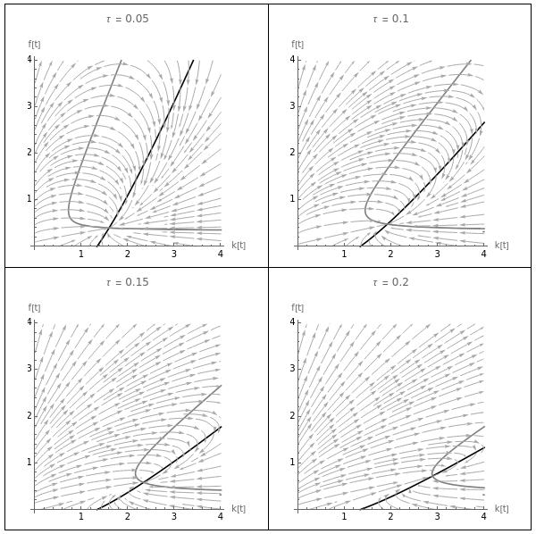
(*Parametrosparasimulaciones1a4condiferentestasasdeinteres*)
In[]:=
simulaciones=Table[{a0.8,γ10.8,σ13,σ23,τx,ω1[t]0.5,ω2[t]0.5},{x,0.05,0.2,0.05}]
Out[]=
{{a0.8,γ10.8,σ13,σ23,τ0.05,ω1[t]0.5,ω2[t]0.5},{a0.8,γ10.8,σ13,σ23,τ0.1,ω1[t]0.5,ω2[t]0.5},{a0.8,γ10.8,σ13,σ23,τ0.15,ω1[t]0.5,ω2[t]0.5},{a0.8,γ10.8,σ13,σ23,τ0.2,ω1[t]0.5,ω2[t]0.5}}
(*Funcionauxiliarparagenerargraficas*)
In[]:=
figeq[parametros_,limsup_:{4,4}]:=Show[ContourPlot[Evaluate[{ec[28],ec[32]}/.parametros],{k[t],0,limsup[[1]]},{f[t],0,limsup[[2]]},ContourStyle{Black,Gray},FrameFalse,AxesTrue,AxesLabel{"k[t]","f[t]"},PlotLabel"τ = "<>ToString[parametros[[5,2]]]],StreamPlot[{ec[26][[2]],ec[27][[2]]}/.parametros,{k[t],0,limsup[[1]]},{f[t],0,limsup[[2]]},StreamStyleGrayLevel[0.66],StreamScale0.13]]
(*Ejemplodeusodelafunciondeplanodefaseylineasnulas*)
In[]:=
figeq[{a0.8,γ10.8,σ13,σ23,τ0.05,ω1[t]0.5,ω2[t]0.5}]
Out[]=
In[]:=
figura4=GraphicsGrid[{{figeq[simulaciones[[1]]],figeq[simulaciones[[2]]]},{figeq[simulaciones[[3]]],figeq[simulaciones[[4]]]}},FrameAll]
Out[]=
(*Parametrosparasimulacion2*)
In[]:=
paramsim2=paramsim1;
In[]:=
paramsim2[[5]]=τ0.10;
In[]:=
paramsim1
Out[]=
{a0.8,γ10.8,σ13,σ23,τ0.05,ω1[t]0.5,ω2[t]0.5}
In[]:=
paramsim2
Out[]=
{a0.8,γ10.8,σ13,σ23,τ0.1,ω1[t]0.5,ω2[t]0.5}
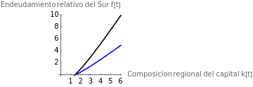
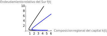
(*Figura5:Impactodeaumentodelatasadeinteresenlineasnulas*)
In[]:=
ec[28]
Out[]=
f[t]
k[t](γ1(-1+ω1[t])+k[t](1-γ1+ω1[t](-1+a+γ1-aω2[t])))
γ1σ1τ(1+k[t])
In[]:=
figura5a=ContourPlot[Evaluate[{ec[28]/.paramsim1,ec[28]/.paramsim2}],{k[t],0,6},{f[t],0,10},ContourStyle{Black,Blue},FrameFalse,AxesTrue,AxesLabel{"Composicion regional del capital k[t]","Endeudamiento relativo del Sur f[t]"},PlotLegends{"τ = "<>ToString[paramsim1[[5,2]]],"τ = "<>ToString[paramsim2[[5,2]]]}]
Out[]=
 |
|
In[]:=
figura5b=ContourPlot[Evaluate[{ec[32]/.paramsim1,ec[32]/.paramsim2}],{k[t],0,6},{f[t],0,10},ContourStyle{Black,Blue},FrameFalse,AxesTrue,AxesLabel{"Composicion regional del capital k[t]","Endeudamiento relativo del Sur f[t]"},PlotLegends{"τ = "<>ToString[paramsim1[[5,2]]],"τ = "<>ToString[paramsim2[[5,2]]]}]
Out[]=
 |
|
(*Simulacion5:casoinestable*)
In[]:=
figura7=figeq[{a0.8,γ10.8,σ13,σ23,τ0.7,ω1[t]0.5,ω2[t]0.5},{20,5}]
Out[]=

(*Estimaciondeumbralparatasadeinteres*)
In[]:=
ec[38]/.{a0.8,γ10.8,σ13,σ23,ω1[t]0.5,ω2[t]0.5}
Out[]=
τ<0.5
(*************************************************************************)(**********Terceraparte:modeloNSDDcompletoyciclosdistributivos**********)(*************************************************************************)
In[]:=
ec[41]={v1'[t]/v1[t]-ρ01+ρl1*l1[t],v2'[t]/v2[t]-ρ02+ρl2*l2[t]};
In[]:=
ec[42]={α1q1'[t]/q1[t],α2q2'[t]/q2[t]};
In[]:=
ec[43]={β1N1'[t]/N1[t],β2N2'[t]/N2[t]};
In[]:=
ec[44]=deduccion2[[1,19]]/.{RuleEqual}
Out[]=
l1[t]
D2[t]k[t]
σ1f[t]N1[t]q1[t]
In[]:=
ec[45]=deduccion2[[1,20]]/.{RuleEqual}
Out[]=
l2[t]
D2[t]
σ2f[t]N2[t]q2[t]
In[]:=
ec[46]=deduccion2[[1,17]]/.{RuleEqual}
Out[]=
v1[t]q1[t]+ω1[t]-aω1[t]
σ1
σ2k[t]
In[]:=
ec[47]=deduccion2[[1,18]]/.{RuleEqual}
Out[]=
v2[t]
aσ2k[t]q2[t]ω1[t]ω2[t]
σ1
In[]:=
ec[48]=(Solve[{D[Log[ec[44][[1]]]Log[ec[44][[2]]],t],ec[25],ec[42][[1]],ec[42][[2]],ec[43][[1]],ec[43][[2]],deduccion2[[1,3]],deduccion2[[1,27]]}/.{RuleEqual},{l1'[t],D2'[t],q1'[t],q2'[t],N1'[t],N2'[t],g1[t],g2[t]}][[1,1]]//FullSimplify)/.{RuleEqual}
Out[]=
′
l1
k[t]l1[t](1-γ1+ω1[t](-1+a+γ1-aω2[t]))
σ1
l1[t][t]
′
k
k[t]
In[]:=
ec[49]=(Solve[{D[Log[ec[45][[1]]]Log[ec[45][[2]]],t],ec[25],ec[42][[1]],ec[42][[2]],ec[43][[1]],ec[43][[2]],deduccion2[[1,3]],deduccion2[[1,27]]}/.{RuleEqual},{l2'[t],D2'[t],q1'[t],q2'[t],N1'[t],N2'[t],g1[t],g2[t]}][[1,1]]//FullSimplify)/.{RuleEqual}
Out[]=
′
l2
l2[t]((α2+β2)σ1+γ1σ1τf[t]+k[t](-1+γ1+ω1[t](1-a-γ1+aω2[t])))
σ1
In[]:=
ec[50]=(Solve[{D[Log[ec[46][[1]]]Log[ec[46][[2]]],t],ec[25],ec[42][[1]],ec[42][[2]],ec[43][[1]],ec[43][[2]],deduccion2[[1,3]],deduccion2[[1,27]],ec[41][[1]]}/.{RuleEqual},{ω1'[t],v1'[t],D2'[t],q1'[t],q2'[t],N1'[t],N2'[t],g1[t],g2[t]}][[1,1]]//FullSimplify)/.{RuleEqual}
Out[]=
′
ω1
k[t](α1+ρ01-ρl1l1[t])(σ1-(-1+a)σ2k[t]ω1[t])-σ1[t]
′
k
(-1+a)σ2
2
k[t]
In[]:=
ec[51]=(Solve[{D[Log[ec[47][[1]]]Log[ec[47][[2]]],t],ec[25],ec[25],ec[42][[1]],ec[42][[2]],ec[43][[1]],ec[43][[2]],deduccion2[[1,3]],deduccion2[[1,27]],ec[41][[2]]}/.{RuleEqual},{ω2'[t],v2'[t],D2'[t],q1'[t],q2'[t],N1'[t],N2'[t],g1[t],g2[t]}][[1,1]]//FullSimplify)/.{RuleEqual}
Out[]=
′
ω2
′
k
k[t]
(α2+ρ02)ω1[t]+[t]
′
ω1
ω1[t]
(*Parametrosparasimulacion6*)
In[]:=
paramsim6={a0.8,γ10.8,σ13,σ23,τ0.05,α10.065,β10.065,α20.065,β20.065,ρ010.2,ρl10.8,ρ020.2,ρl20.8};
In[]:=
valiniciales={ω1[0]0.5,ω2[0]0.5,l1[0]0.3,l2[0]0.3,k[0]2,f[0]0.5};
In[]:=
sistemadin={ec[48],ec[49],ec[50],ec[51],ec[26],ec[27]};
In[]:=
solucionnum1=NDSolve[Join[sistemadin,valiniciales]/.paramsim6,{l1,l2,ω1,ω2,k,f},{t,0,1000}];
In[]:=
soln1l1=solucionnum1[[1,1,2]];
In[]:=
soln1l2=solucionnum1[[1,2,2]];
In[]:=
soln1ω1=solucionnum1[[1,3,2]];
In[]:=
soln1ω2=solucionnum1[[1,4,2]];
In[]:=
soln1k=solucionnum1[[1,5,2]];
In[]:=
soln1f=solucionnum1[[1,6,2]];
In[]:=
(*Trayectoriaseneltiempo*)
In[]:=
figura8a=Plot[soln1l1[t],{t,0,200},PlotLabel"Tasa de empleo del Norte l1[t]",PlotStyleGray];
In[]:=
figura8b=Plot[soln1l2[t],{t,0,200},PlotLabel"Tasa de empleo del Sur l2[t]",PlotStyleGray];
In[]:=
figura8c=Plot[soln1ω1[t],{t,0,200},PlotLabel"Participacion salarial en el Norte ω1[t]",PlotStyleGray];
In[]:=
figura8d=Plot[soln1ω2[t],{t,0,200},PlotLabel"Participacion salarial en el Sur ω2[t]",PlotStyleGray];
In[]:=
figura8e=Plot[soln1k[t],{t,0,200},PlotLabel"Composicion sectorial del capital k[t]",PlotStyleGray];
In[]:=
figura8f=Plot[soln1f[t],{t,0,200},PlotLabel"Endeudamiento relativo del Sur f[t]",PlotStyleGray];
In[]:=
figura8=GraphicsGrid[{{figura8a,figura8b},{figura8c,figura8d},{figura8e,figura8f}},FrameAll,AspectRatioFull]
Out[]=

(*Ciclosdistributivossimultaneos*)
In[]:=
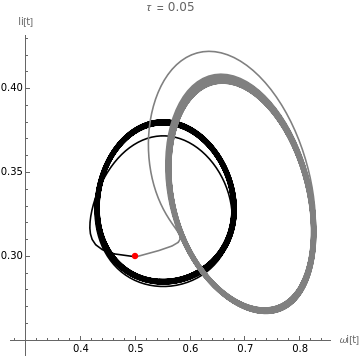
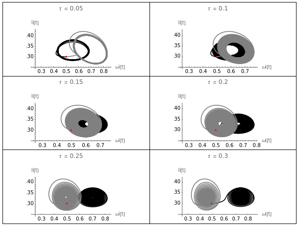
tasaciclos[condiniciales_,parametros_,aspecto_:1,origen_:{0,0},periodofin_:1000,sistema_:sistemadin]:=Show[ParametricPlot[Evaluate[{ω1[t],l1[t]}/.NDSolve[Join[sistema,condiniciales]/.parametros,{l1,l2,ω1,ω2,k,f},{t,0,periodofin}]],{t,0,periodofin},AspectRatioaspecto,PlotStyleBlack,AxesOriginorigen],ParametricPlot[Evaluate[{ω2[t],l2[t]}/.NDSolve[Join[sistema,condiniciales]/.parametros,{l1,l2,ω1,ω2,k,f},{t,0,periodofin}]],{t,0,periodofin},AspectRatioaspecto,PlotStyleGray],Graphics[{PointSize[0.02],Red,Point[{condiniciales[[1,2]],condiniciales[[3,2]]}]}],PlotRangeAll,AxesLabel{"ωi[t]","li[t]"},PlotLabel"τ = "<>ToString[parametros[[5,2]]]]
In[]:=
valiniciales
Out[]=
{ω1[0]0.5,ω2[0]0.5,l1[0]0.3,l2[0]0.3,k[0]2,f[0]0.5}
In[]:=
paramsim6
Out[]=
{a0.8,γ10.8,σ13,σ23,τ0.05,α10.065,β10.065,α20.065,β20.065,ρ010.2,ρl10.8,ρ020.2,ρl20.8}
In[]:=
figura9=Legended[tasaciclos[valiniciales,paramsim6,1,{0.3,0.25}],LineLegend[{Black,Gray,Red},{"Ciclo del Norte","Ciclo del Sur","Valor inicial"}]]
Out[]=
 |
|
(*Efectodelatasadeinteressobrelosciclos*)
In[]:=
simtasaciclos=Table[{a0.8,γ10.8,σ13,σ23,τx,α10.065,β10.065,α20.065,β20.065,ρ010.2,ρl10.8,ρ020.2,ρl20.8},{x,0.05,0.3,0.05}]
Out[]=
{{a0.8,γ10.8,σ13,σ23,τ0.05,α10.065,β10.065,α20.065,β20.065,ρ010.2,ρl10.8,ρ020.2,ρl20.8},{a0.8,γ10.8,σ13,σ23,τ0.1,α10.065,β10.065,α20.065,β20.065,ρ010.2,ρl10.8,ρ020.2,ρl20.8},{a0.8,γ10.8,σ13,σ23,τ0.15,α10.065,β10.065,α20.065,β20.065,ρ010.2,ρl10.8,ρ020.2,ρl20.8},{a0.8,γ10.8,σ13,σ23,τ0.2,α10.065,β10.065,α20.065,β20.065,ρ010.2,ρl10.8,ρ020.2,ρl20.8},{a0.8,γ10.8,σ13,σ23,τ0.25,α10.065,β10.065,α20.065,β20.065,ρ010.2,ρl10.8,ρ020.2,ρl20.8},{a0.8,γ10.8,σ13,σ23,τ0.3,α10.065,β10.065,α20.065,β20.065,ρ010.2,ρl10.8,ρ020.2,ρl20.8}}
In[]:=
figura10=GraphicsGrid[{{tasaciclos[valiniciales,simtasaciclos[[1]],0.5,{0.25,0.25}],tasaciclos[valiniciales,simtasaciclos[[2]],0.5,{0.25,0.25}]},{tasaciclos[valiniciales,simtasaciclos[[3]],0.5,{0.25,0.25}],tasaciclos[valiniciales,simtasaciclos[[4]],0.5,{0.25,0.25}]},{tasaciclos[valiniciales,simtasaciclos[[5]],0.5,{0.25,0.25}],tasaciclos[valiniciales,simtasaciclos[[6]],0.5,{0.25,0.25}]}},FrameAll]
Out[]=
(*ComparacionparticipacionessalarialesNorte-Surytasadeinteres*)
In[]:=
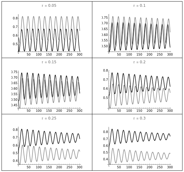
tasaparticipaciones[condiniciales_,parametros_,periodofin_:300,sistema_:sistemadin]:=Plot[Evaluate[{ω1[t],ω2[t]}/.NDSolve[Join[sistema,condiniciales]/.parametros,{l1,l2,ω1,ω2,k,f},{t,0,periodofin}]],{t,0,periodofin},PlotStyle{Black,Gray},PlotLabel"τ = "<>ToString[parametros[[5,2]]]]
In[]:=
figura11=GraphicsGrid[{{tasaparticipaciones[valiniciales,simtasaciclos[[1]]],tasaparticipaciones[valiniciales,simtasaciclos[[2]]]},{tasaparticipaciones[valiniciales,simtasaciclos[[3]]],tasaparticipaciones[valiniciales,simtasaciclos[[4]]]},{tasaparticipaciones[valiniciales,simtasaciclos[[5]]],tasaparticipaciones[valiniciales,simtasaciclos[[6]]]}},FrameAll]
Out[]=
(*Comparacionciclosestableseinestables*)
In[]:=
paramsim12={a0.8,γ10.8,σ13,σ23,τ0.05,α10.065,β10.065,α20.065,β20.065,ρ010.2,ρl10.9,ρ020.2,ρl20.8};
In[]:=
paramsim13={a0.8,γ10.8,σ13,σ23,τ0.05,α10.065,β10.065,α20.065,β20.065,ρ010.2,ρl10.8,ρ020.2,ρl20.9};
In[]:=
ciclosdeuda[condiniciales_,parametros_,periodofin_:500,sistema_:sistemadin]:=Plot[Evaluate[{f[t]}/.NDSolve[Join[sistema,condiniciales]/.parametros,{l1,l2,ω1,ω2,k,f},{t,0,periodofin}]],{t,0,periodofin},PlotStyleGray,AxesLabel{"t","f[t]"},PlotLabel"ρl1 = "<>ToString[parametros[[11,2]]]<>"; ρl2 = "<>ToString[parametros[[13,2]]]]
In[]:=
GraphicsRow[{ciclosdeuda[valiniciales,paramsim12],ciclosdeuda[valiniciales,paramsim13]}]
Out[]=

Cite this as: John Cajas Guijarro, "Debt, Power, and Cycles: A North-South Model of Debt and Distribution (NSDD)" from the Notebook Archive (2023), https://notebookarchive.org/2023-12-cxl4iz7
Download
