Working Material

Redefining the Homeostatic Role of HIFs

Clemente Fernandez Arias

Author

Clemente Fernandez Arias

Title

Redefining the Homeostatic Role of HIFs

Description

Supplementary material for "Redefining the role of Hypoxia-inducible factors (HIFs) in oxygen homeostasis"

Redefining the Homeostatic Role of HIFs

Supplementary material to
“Redefining the role of Hypoxia Inducible Factors (HIFs) in oxygen homeostasis” (2024)

Clemente F. Arias
1*

, Francisco J. Acosta
2

, Federica Bertocchini
3

, and Cristina Fernández-Arias
4*

Grupo Interdisciplinar de Sistemas Complejos (GISC), 28040 Madrid, Spain.

Departamento de Ecología, Universidad Complutense de Madrid, 28040 Madrid, Spain.

Plasticentropy, 51100 Reims, France.

Departamento de Inmunología, Universidad Complutense de Madrid, 28040 Madrid, Spain.

*Corresponding authors: CFA: tifar@ucm.es, CrF-A: crifer25@ucm.es

This notebook contains the code used to generate Figs. 3-5 in the main text.

Model definition

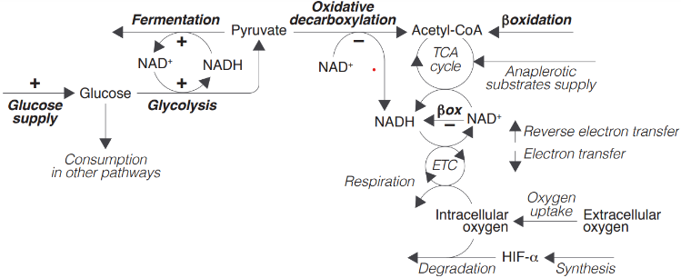
In this section, we formulate a mathematical version of the following conceptual model (shown in Figure 2 in the main text):

The variables and parameters of this model will be denoted as indicated below:

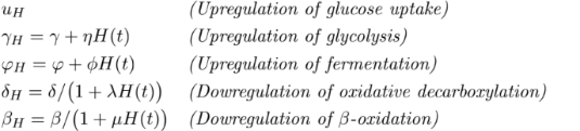
The concentration of glucose, pyruvate, acetyl-CoA, intracellular oxygen, and HIF-α are labeled as glu , pyr, ace, oxy, and hif respectively; nad and nadH represent the concentration of NAD+ and NADH respectively; and etc and etcH that of the oxidized and reduced components of the electron transport chain respectively. HIFs regulation is modeled as:

The previous conceptual model can be formalized within the framework of the law of mass action as shown in Supplementary Material A. The corresponding equations can be expressed as follows:

Clear[model];model[sH_,EO2_,mG_,mA_,mF_]:={glu'[t]mG+uHhif[t]-ωglu[t]-(γ+ηhif[t])glu[t]nad[t]^2,pyr'[t]2(γ+ηhif[t])glu[t]nad[t]^2-δpyr[t]nad[t]/(1+λhif[t])-(φ+ϕhif[t])pyr[t]nadH[t],ace'[t]mFβnad[t]/(1+μhif[t])+δpyr[t]nad[t]/(1+λhif[t])-τace[t]nad[t]^3,nad'[t]-3τace[t]nad[t]^3-δpyr[t]nad[t]/(1+λhif[t])+ϵnadH[t]etc[t]-mFβnad[t]/(1+μhif[t])-mAαnad[t]+(φ+ϕhif[t])pyr[t]nadH[t]-2(γ+ηhif[t])glu[t]nad[t]^2-ϵetcH[t]nad[t],nadH'[t]3τace[t]nad[t]^3+mFβnad[t]/(1+μhif[t])+mAαnad[t]+δpyr[t]nad[t]/(1+λhif[t])-ϵnadH[t]etc[t]-(φ+ϕhif[t])pyr[t]nadH[t]+2(γ+ηhif[t])glu[t]nad[t]^2+ϵetcH[t]nad[t],etc'[t]-ϵnadH[t]etc[t]+2ρetcH[t]^2oxy[t]+ϵetcH[t]nad[t],etcH'[t]ϵnadH[t]etc[t]-2ρetcH[t]^2oxy[t]-ϵetcH[t]nad[t],hif'[t]sH-kHhif[t]oxy[t],oxy'[t]υ(EO2-oxy[t])-ρetcH[t]^2oxy[t]-kHhif[t]oxy[t],glu[0]0,pyr[0]1,ace[0]0,etc[0]0,etcH[0]Cetc,nadH[0]0,nad[0]Cnad,hif[0]0,oxy[0]1};

variables={glu[t],pyr[t],hif[t],oxy[t],nadH[t],nad[t],ace[t],etcH[t],etcH[t]};

The previous equations simulate the dynamics of the conceptual model shown in Figure 2 taking as inputs the rate of HIF-α synthesis (sH), extracellular oxygen tensions (EO2), and the metabolic supply of glucose (mG), anaplerotic substrates for the TCA cycle (mA), and fatty acids for β-oxidation (mF).

Clear[solution];solution[sH_,EO2_,mG_,mA_,mF_]:=NDSolve[model[sH,EO2,mG,mA,mF]/.parameters,variables,{t,0,200000},Method->{"EquationSimplification"->"Residual"}];

Numerical simulations range from t = 0 to t = 200000, which allows the system to stabilize and reach its steady state.

parameters={uH.5,ω3,γ.8,η.1,δ1.5,φ0.01,ϕ2.,λ.2,μ.2,τ.5,ϵ5,kH.5,υ0.8,ρ1,α->1,β->1,Cnad->100,Cetc->500};

The parameters represent the rates of the metabolic pathways considered in the model, as shown in Model 1, except for Cnad and Cetc, which denote the capacity of the NAD+/NADH cycle and the electron transport chain respectively. The values of the parameters have been arbitrarily chosen to illustrate the behavior of the conceptual model outlined above.

Figures

Figure 3

In this section, we perform numerical simulations of the model for a range of values of extracellular oxygen levels (20<= EO2<=10000) and glucose metabolic supply (20<=mG<=1000), assuming that there is no HIFs-mediated regulation (i.e. that sH=0). In these simulations, the supply of anaplerotic substrates and fatty acids is constant: mA = mF = 10. These values, as well as the range of extracellular tensions and glucose supply, are chosen arbitrarily to illustrate the dynamics of the model.

Clear[resultsFig3];resultsFig3=Flatten[Table[{{EO2,mG},(solution[0,EO2,mG,10,10]/.t200000)[[1,All,2]]},{EO2,20,10000,20},{mG,20,1000,20}],1];

Clear[data];Table[data[variables[[j]]]=Table[Flatten[{resultsFig3[[i,1]],resultsFig3[[i,2,j]]}],{i,1,Length[resultsFig3]}],{j,1,9}];

The data are now interpolated:

Clear[interpolation];Map[(interpolation[#]=Interpolation[data[#],InterpolationOrder2])&,variables];

and plotted:

Fig3A=Plot3D[interpolation[etcH[t]][EO2,mG],{EO2,20,10000},{mG,20,1000},MeshFunctions{#2&},Mesh7,PlotPoints100,TicksNone,ImageSize150,PlotLabel->"ECTH (%)"]

Fig3B=Plot3D[interpolation[nadH[t]][sO,sG],{sO,20,10000},{sG,20,1000},MeshFunctions{#2&},Mesh7,PlotPoints100,TicksNone,ImageSize150,PlotLabel->"NADH (%)"]

Fig3C=Plot3D[Log[interpolation[ace[t]][sO,sG]],{sO,20,9000},{sG,20,1000},MeshFunctions{#2&},Mesh7,TicksNone,ImageSize150,PlotRangeAll,PlotLabel->"Acetyl-CoA"]

Figures 3.C and E show numerical simulations of the model for a range of values of extracellular oxygen (EO2) and metabolic supply (m) and three different rates of HIF-α synthesis. The metabolic supply of glucose, fatty acids, and anaplerotic substrates is assumed to increase linearly with the value of metabolic supply m (mG = m, mA = m/20, and mF = m/15). This is an arbitrary choice to illustrate the dynamics of the model. The figures show the steady-state value of NADH (%), which is calculated as 100 nadH/(nad + nadH).

resultsFig3C=Interpolation[Flatten[Table[{EO2,m,(nadH[t]/.solution[0,EO2,m,m/20,m/15]/.t200000)[[1]]},{EO2,50,9000,50},{m,50,1100,50}],1],InterpolationOrder->2];

ContourPlot[resultsFig3C[EO2,m],{EO2,50,9000},{m,50,1100},FrameTicksNone,ImageSize130,Contours8,ColorFunctionGrayLevel,AspectRatio1,PlotRangeAll]

resultsFig3ELeft=Interpolation[Flatten[Table[{EO2,m,(nadH[t]/.solution[0.1,EO2,m,m/20,m/15]/.t200000)[[1]]},{EO2,50,9000,50},{m,50,1100,50}],1],InterpolationOrder->2];

ContourPlot[resultsFig3ELeft[EO2,m],{EO2,50,9000},{m,50,1100},FrameTicksNone,ImageSize130,Contours8,ColorFunctionGrayLevel,AspectRatio1,PlotRangeAll]

resultsFig3ERight=Interpolation[Flatten[Table[{EO2,m,(nadH[t]/.solution[2.,EO2,m,m/20,m/15]/.t200000)[[1]]},{EO2,50,9000,50},{m,50,1100,50}],1],InterpolationOrder->2];

ContourPlot[resultsFig3ERight[EO2,m],{EO2,50,9000},{m,50,1100},FrameTicksNone,ImageSize130,Contours8,ColorFunctionGrayLevel,AspectRatio1,PlotRangeAll]

Figure 4

Figure 4 shows the behavior of the model for a range of values of extracellular oxygen values (50<=EO2<=10000).

extracellularOxygen=Table[EO2,{EO2,50,10000,50}];

Metabolic supply of glucose, anaplerotic substrates, and fatty acids is constant (mG = 1000, mA = mF = 10).
Numerical simulations of the model without HIFs regulation (sH = 0):

withoutHIFs=Map[solution[0,#,1000,10,10]&,extracellularOxygen];

Numerical simulations of the model with HIFs regulation (sH = 10):

withHIFs=Map[solution[10,#,1000,10,10]&,extracellularOxygen];

The following figures represent the dependence of the system’s steady-state on extracellular oxygen levels. Results with and without HIFs regulation are shown in orange and blue respectively.

Fig4A=Show[ListLinePlot[Transpose[{extracellularOxygen,Flatten[Map[hif[t]/.#/.t200000&,withHIFs]]}],PlotRange{0,50},PlotStyleOrange],ImageSize150,Ticks{Table[EO2,{EO2,0,10000,3000}],Table[hif,{hif,0,50,20}]},PlotLabel->"HIFα"]

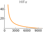
Fig4B=Show[ListLinePlot[Transpose[{extracellularOxygen,Flatten[Map[(φ+ϕhif[t])pyr[t]nadH[t]/.parameters/.#/.t200000&,withHIFs]]}],PlotStyleOrange,PlotRange{0,3200}],ListLinePlot[Transpose[{extracellularOxygen,Flatten[Map[(φ+ϕhif[t])pyr[t]nadH[t]/.parameters/.#/.t200000&,withoutHIFs]]}]],ImageSize150,Ticks{Table[EO2,{EO2,0,10000,3000}],Table[ferm,{ferm,0,3000,1000}]},PlotLabel->"Fermentation"]

Fig4C=Show[ListLinePlot[Transpose[{extracellularOxygen,Flatten[Map[δpyr[t]nad[t]/(1+λhif[t])/.parameters/.#/.t200000&,withHIFs]]}],PlotStyleOrange],ListLinePlot[Transpose[{extracellularOxygen,Flatten[Map[δpyr[t]nad[t]/(1+λhif[t])/.parameters/.#/.t200000&,withoutHIFs]]}]],ImageSize150,Ticks{Table[EO2,{EO2,0,10000,3000}],Table[oxDec,{oxDec,0,2000,400}]},PlotLabel->"Oxidative\ndecarboxylation"]

Fig4D=Show[ListLinePlot[Transpose[{extracellularOxygen,Flatten[Map[γglu[t]nad[t]^2/.parameters/.#/.t200000&,withoutHIFs]]}]],ListLinePlot[Transpose[{extracellularOxygen,Flatten[Map[(γ+ηhif[t])glu[t]nad[t]^2/.parameters/.#/.t200000&,withHIFs]]}],PlotStyleOrange,PlotRange{0,1500}],ImageSize150,PlotRange{0,1500},Ticks{Table[EO2,{EO2,0,10000,3000}],Table[gly,{gly,0,1500,500}]},PlotLabel->"Glycolysis"]

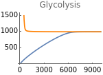
Fig4E=Show[ListLinePlot[Transpose[{extracellularOxygen,Flatten[Map[ρetcH[t]^2oxy[t]/.parameters/.#/.t200000&,withHIFs]]}],PlotStyleOrange],ListLinePlot[Transpose[{extracellularOxygen,Flatten[Map[ρetcH[t]^2oxy[t]/.parameters/.#/.t200000&,withoutHIFs]]}]],ImageSize150,Ticks{Table[EO2,{EO2,0,10000,3000}],Table[resp,{resp,1000,7000,2000}]},PlotRange{0,7000},PlotLabel->"Respiration"]

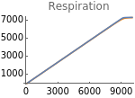
Fig4F=Show[ListLinePlot[Transpose[{extracellularOxygen,Flatten[Map[etcH[t]/5/.#/.t200000&,withHIFs]]}],PlotStyleOrange,PlotRangeAll],ListLinePlot[Transpose[{extracellularOxygen,Flatten[Map[etcH[t]/5/.#/.t200000&,withoutHIFs]]}],PlotRangeAll],ImageSize150,PlotRange{0,100},AxesOrigin{0,0},Ticks{Table[EO2,{EO2,0,10000,3000}],Table[etcH,{etcH,0,100,20}]},PlotLabel->"ETCH(%)"]

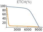
Fig4G=Show[ListLinePlot[Transpose[{extracellularOxygen,Flatten[Map[nadH[t]/.#/.t200000&,withHIFs]]}],PlotStyleOrange,PlotRangeAll],ListLinePlot[Transpose[{extracellularOxygen,Flatten[Map[nadH[t]/.#/.t200000&,withoutHIFs]]}]],ImageSize150,PlotRange{0,100},Ticks{Table[EO2,{EO2,0,10000,3000}],Table[NADH,{NADH,0,200,20}]},PlotLabel->"NADH(%)"]

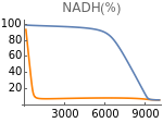
Fig4H=Show[ListLinePlot[Transpose[{extracellularOxygen,Flatten[Map[ace[t]/.#/.t200000&,withHIFs]]}],PlotStyleOrange],ListLinePlot[Transpose[{extracellularOxygen,Flatten[Map[ace[t]/.#/.t200000&,withoutHIFs]]}],PlotRangeAll],ImageSize150,PlotRange{0,.03},Ticks{Table[EO2,{EO2,0,10000,3000}],Table[ace,{ace,0,.03,.01}]},PlotLabel->"Acetyl-CoA"]

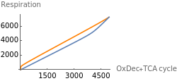
Fig4I represents the dependence of respiration on the entry of electrons in the aerobic pathway. Results with and without HIFs regulation are shown in orange and blue respectively.

Fig4I=Show[ListLinePlot[Transpose[{Flatten[Map[(δpyr[t]nad[t]/(1+λhif[t])+τace[t]nad[t]^3)/.parameters/.#/.t200000&,withHIFs]],Flatten[Map[(ρetcH[t]^2oxy[t])/.parameters/.#/.t200000&,withHIFs]]}],PlotStyleOrange,PlotRangeAll],ListLinePlot[Transpose[{Flatten[Map[(δpyr[t]nad[t]/(1+λhif[t])+τace[t]nad[t]^3)/.parameters/.#/.t200000&,withoutHIFs]],Flatten[Map[(ρetcH[t]^2oxy[t])/.parameters/.#/.t200000&,withoutHIFs]]}]],ImageSize250,PlotRangeAll,Ticks{Table[aerobic,{aerobic,0,40000,1500}],Table[resp,{resp,0,6000,2000}]},AxesLabel->{"OxDec+TCA cycle","Respiration"}]

The following figures represent the dependence of fermentation and glycolysis on the rate of HIF-α synthesis:

Clear[resultsFigs4JK];resultsFigs4JK=Table[solution[sH,400,1000,10,10],{sH,0,20,.05}];

Fig4J=Show[ListLinePlot[Transpose[{Table[sH,{sH,0,20,.05}],Flatten[Map[(φ+ϕhif[t])pyr[t]nadH[t]/.parameters/.#/.t200000&,resultsFigs4JK]]}],PlotRangeAll,PlotStyleOrange],ImageSize150,PlotRange{0,8000},Ticks{Table[sH,{sH,0,20,5}],Table[ferm,{ferm,0,25000,2000}]},PlotLabel->"Fermentation"]

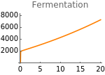
Fig4K=Show[ListLinePlot[Transpose[{Table[sH,{sH,0,20,.05}],Flatten[Map[(γ+ηhif[t])glu[t]nad[t]^2/.parameters/.#/.t200000&,resultsFigs4JK]]}],PlotRangeAll,PlotStyleOrange],ImageSize150,PlotRange{0,4000},Ticks{Table[sH,{sH,0,20,5}],Table[gly,{gly,0,4000,1000}]},PlotLabel->"Glycolysis"]

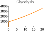
Figure 5

Figure 5 shows the response of the model to changes in metabolic supply (m). The input of glucose, fatty acids, and anaplerotic substrates into the system increases linearly with the value of metabolic supply m (mG = m, mA = m/20, and mF = m/15). Extracellular oxygen tension is constant (EO2=4000).

metabolicSupply=Table[m,{m,0,3000,2}];

Numerical simulations of the model without HIFs regulation (sH = 0):

withoutHIFs=Map[solution[0,4000,#,#/20,#/15]&,metabolicSupply];

Numerical simulations of the model with HIFs regulation (sH = 10):

withHIFs=Map[solution[10,4000,#,#/20,#/15]&,metabolicSupply];

The following figures show the dependence of the system’s steady-state on metabolic supply. Results with and without HIFs regulation are shown in orange and blue respectively.

Fig5A=Show[ListLinePlot[Transpose[{metabolicSupply,Flatten[Map[hif[t]/.parameters/.#/.t200000&,withHIFs]]}],PlotRangeAll,PlotStyleOrange],ImageSize150,PlotRange{0,500},Ticks{Table[m,{m,0,3000,1000}],Table[hif,{hif,0,500,150}]},PlotLabel->"HIF-α"]

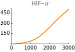
Fig5B=Show[ListLinePlot[Transpose[{metabolicSupply,Flatten[Map[etcH[t]/5/.parameters/.#/.t200000&,withHIFs]]}],PlotRangeAll,PlotStyleOrange],ListLinePlot[Transpose[{metabolicSupply,Flatten[Map[etcH[t]/5/.parameters/.#/.t200000&,withoutHIFs]]}],PlotRangeAll],ImageSize150,PlotRange{0,100},Ticks{Table[m,{m,0,3000,1000}],Table[NADH,{NADH,0,100,20}]},PlotLabel->"NADH (%)"]

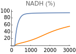
Fig5C=Show[ListLinePlot[Transpose[{metabolicSupply,Flatten[Map[δpyr[t]nad[t]/(1+λhif[t])/.parameters/.#/.t200000&,withHIFs]]}],PlotStyleOrange,PlotRangeAll],ListLinePlot[Transpose[{metabolicSupply,Flatten[Map[δpyr[t]nad[t]/(1+λhif[t])/.parameters/.#/.t200000&,withoutHIFs]]}],PlotRangeAll],ImageSize150,PlotRange{0,1100},Ticks{Table[m,{m,0,3000,1000}],Table[oxDec,{oxDec,0,4000,250}]},PlotLabel->"Oxidative\ndecarboxylation"]

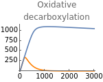
Fig5D=Show[ListLinePlot[Transpose[{metabolicSupply,Flatten[Map[τace[t]nad[t]^3/.parameters/.#/.t200000&,withHIFs]]}],PlotStyleOrange,PlotRangeAll],ListLinePlot[Transpose[{metabolicSupply,Flatten[Map[τace[t]nad[t]^3/.parameters/.#/.t200000&,withoutHIFs]]}],PlotRangeAll],ImageSize150,Ticks{Table[m,{m,0,3000,1000}],Table[tca,{tca,0,2000,400}]},PlotLabel->"TCA cycle"]

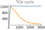
Fig5E=Show[Show[ListLinePlot[Transpose[{metabolicSupply,Flatten[Map[γglu[t]nad[t]^2/.parameters/.#/.t200000&,withHIFs]]}]],ImageSize150,PlotRangeAll],ListLinePlot[Transpose[{metabolicSupply,Flatten[Map[(γ+ηhif[t])glu[t]nad[t]^2/.parameters/.#/.t200000&,withoutHIFs]]}],PlotStyleOrange],ImageSize150,PlotRange{0,800},Ticks{Table[m,{m,0,3000,1000}],Table[gly,{gly,0,800,200}]},PlotLabel->"Glycolysis"]

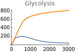
Fig5F=Show[ListLinePlot[Transpose[{metabolicSupply,Flatten[Map[ϕhif[t]pyr[t]nadH[t]+φpyr[t]nadH[t]/.parameters/.#/.t200000&,withHIFs]]}],PlotRangeAll,PlotStyleOrange],ListLinePlot[Transpose[{metabolicSupply,Flatten[Map[ϕhif[t]pyr[t]nadH[t]+φpyr[t]nadH[t]/.parameters/.#/.t200000&,withoutHIFs]]}],PlotRangeAll],ImageSize150,PlotRange{0,7000},Ticks{Table[m,{m,0,3000,1000}],Table[fer,{fer,0,7000,2000}]},PlotLabel->"Fermentation"]

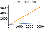
Figure 5.G shows lactate production as a function of metabolic supply for three different values of extracellular oxygen tension (EO2 = 1000, 4000, and 20000). These values are chosen arbitrarily to represent low, intermediate, and high values of oxygen availability.

withHIFsHypoxia=Map[solution[10,1000,#,#/20,#/15]&,metabolicSupply];

withHIFsNormoxia=Map[solution[10,20000,#,#/20,#/15]&,metabolicSupply];

Fig5G=Show[ListLinePlot[Transpose[{metabolicSupply,Flatten[Map[ϕhif[t]pyr[t]nadH[t]+φpyr[t]nadH[t]/.parameters/.#/.t200000&,withHIFsHypoxia]]}],PlotRangeAll,PlotStyleGreen],ListLinePlot[Transpose[{metabolicSupply,Flatten[Map[ϕhif[t]pyr[t]nadH[t]+φpyr[t]nadH[t]/.parameters/.#/.t200000&,withHIFs]]}],PlotRangeAll,PlotStyleOrange],ListLinePlot[Transpose[{metabolicSupply,Flatten[Map[ϕhif[t]pyr[t]nadH[t]+φpyr[t]nadH[t]/.parameters/.#/.t200000&,withHIFsNormoxia]]}],PlotRangeAll],ImageSize150,PlotRange{0,11000},Ticks{Table[m,{m,0,3000,1000}],Table[fer,{fer,0,12000,3000}]},PlotLabel->"Lactate production"]

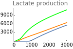
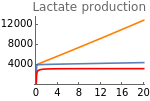
Figure 5.H shows the changes in lactate production with the rate of HIF-α synthesis (sH) for three values of extracellular oxygen tensions (EO2 = 1000, 4000, and 20000). These values are chosen arbitrarily to represent low, intermediate, and high values of oxygen availability.

hypoxia=Table[solution[sH,1000,2000,2000/20,2000/15],{sH,0,20,.05}];

physioxia=Table[solution[sH,4000,2000,2000/20,2000/15],{sH,0,20,.05}];

normoxia=Table[solution[sH,20000,2000,2000/20,2000/15],{sH,0,20,.05}];

Fig5H=Show[ListLinePlot[Transpose[{Table[sH,{sH,0,20,.05}],Flatten[Map[(ϕhif[t]+φ)pyr[t]nadH[t]/.parameters/.#/.t200000&,hypoxia]]}],PlotStyleOrange,PlotRangeAll],ListLinePlot[Transpose[{Table[sH,{sH,0,20,.05}],Flatten[Map[(ϕhif[t]+φ)pyr[t]nadH[t]/.parameters/.#/.t200000&,physioxia]]}],PlotRangeAll],ListLinePlot[Transpose[{Table[sH,{sH,0,20,.05}],Flatten[Map[(ϕhif[t]+φ)pyr[t]nadH[t]/.parameters/.#/.t200000&,normoxia]]}],PlotStyleRed,PlotRangeAll],ImageSize150,Ticks{Table[sH,{sH,0,20,4}],Table[sO,{sO,0,12000,4000}]},PlotRangeAll,PlotLabel->"Lactate production"]

Cite this as: Clemente Fernandez Arias, "Redefining the Homeostatic Role of HIFs" from the Notebook Archive (2024), https://notebookarchive.org/2024-02-cvllu1f

Redefining the Homeostatic Role of HIFs

Supplementary material to ​​“Redefining the role of Hypoxia Inducible Factors (HIFs) in oxygen homeostasis” (2024)

Clemente F. Arias1*​, Francisco J. Acosta2​, Federica Bertocchini3​, and Cristina Fernández-Arias4*​

​This notebook contains the code used to generate Figs. 3-5 in the main text.​

Model definition

Figures

Figure 3

Figure 4

Figure 5

Supplementary material to
“Redefining the role of Hypoxia Inducible Factors (HIFs) in oxygen homeostasis” (2024)

Clemente F. Arias
1*

, Francisco J. Acosta
2

, Federica Bertocchini
3

, and Cristina Fernández-Arias
4*

This notebook contains the code used to generate Figs. 3-5 in the main text.