Computing the slope of a logarithmic curvature graph
Author
Norimasa Yoshida
Title
Computing the slope of a logarithmic curvature graph
Description
This notebook provides a code for computing the slope of a logarithmic curvature graph. Although examples are a logarithmic spiral and a hyperbolic spiral, we can compute the slopes the logarithmic curvature graphs of any curves, not only 2D but also 3D curves.
Category
Academic Articles & Supplements
Keywords
logarithmic curvature graph, log-aesthetic curves, Clothoid, Nielsen's spiral, logarithmic spiral, circle involute
URL
http://www.notebookarchive.org/2024-06-1ucl8i6/
DOI
https://notebookarchive.org/2024-06-1ucl8i6
Date Added
2024-06-04
Date Last Modified
2024-06-04
File Size
61.41 kilobytes
Supplements
Rights
Redistribution rights reserved

Computing the slope of a logarithmic curvature graph
Norimasa Yoshida
Nihon University
yoshida.norimasa@nihon-u.ac.jp
Nihon University
yoshida.norimasa@nihon-u.ac.jp
This notebook provides a code for computing the slope of a logarithmic curvature graph (LCG) , which we call a. a can be computed at any point of any curve, except at dk/ds is zero . If a is equal to -1, 0, 1, or 2, the curve is the Clothoid (Cornu’s spiral), Nielsen’s spiral, a logarithmic spiral, or the circle involute, respectively. A curve with constant a is called a log-aesthetic curves [3]. At the time when the paper [3] was published, log-aesthetic curves were called Aesthetic curves. In CAD conference of 2007, just before my presentation of [4], Prof. Carlo H. Séquin of U. C. Berkely recommended us to use log-aesthetic curves. Then we started using log-aesthetic curves.
For the details, refer to [1]. For the details about logarithmic curvature graphs, refer to [2]. The original idea of logarithmic curvature graphs comes from log-aesthetic curves [3]. Original idea of log-aesthetic curves comes from Harada [5]. The general equation is derived by Miura [6]. In [3], we clarified overall shapes and various characteristics. We also proposed a method to draw a log-aesthetic curve segment like a quadratic Bézier curve.
For 3D curves, not only a but also b, which is the slope of a logarithmic torsion graph, can be computed. By slightly modifying the code, we can also compute b. For 3D curves, the determinant in computing the curvature should be replaced by the cross product.
References:
[1] Norimasa Yoshida and Takafumi Saito, Shape Information of Curves and its Visualization using Two-tone Pseudo Coloring, Computer-Aided Design and Applications, Vol. 21, No.1, pp.11-28, Jan. 2024. https://doi.org/10.14733/cadaps.2024.11-28
[2] Noriamsa Yoshida, Ryo Fukuda, Takafumi Saito, Logarithmic Curvature and Torsion Graphs, in Mathematical Methods for Curves and Surfaces 2008 edited by Daehlen et al., LNCS 5862, Springer, pp.434-443, 2010. https://doi.org/10.1007/978-3-642-11620-9_28
[3] Norimasa Yoshida and Takafumi Saito, Interactive Aesthetic Curve Segments, The Visual Computer (Pacific Graphics), Vol. 22, No.9-11, pp.896-905, 2006. https://doi.org/10.1007/s00371-006-0076-5
[4] Norimasa Yoshida and Takafumi Saito, Quasi-Aesthetic Curves in Rational Cubic Bezier Forms, Computer-Aided Design & Applications, Vol. 4, Nos. 1-4, pp.477-486, 2007. https://doi.org/10.1080/16864360.2007.10738567
Norimasa Yoshida (Nihon University)
Norimasa Yoshida (Nihon University)
[5] T. Harada, F. Yoshimoto, M. Moriyama, An aesthetic curve in the field of industrial design, Proceedings of IEEE Symposium on Visual Languages, pp. 38–47. IEEE Computer Society Press, 1999. https://doi.org/10.1109/VL.1999.795873
[6] K. T. Miura, A general equation of aesthetic curves and its self-affinity, Computer Aided Design and Applications, Vol. 3, Nos 1-4, pp. 457-464, 2006. https://doi.org/10.1080/16864360.2006.10738484
In[]:=
normfd[f_][t_]:=Sqrt[D[f[x],x].D[f[x],x]]/.x->t
In[]:=
kappa[f_][t_]:=Sqrt[Det[{D[f[x],{x,1}],D[f[x],{x,2}]}]^2]/normfd[f][x]^3/.xt
In[]:=
dkds[f_][t_]:=D[kappa[f][x],x]/normfd[f][x]/.xt
In[]:=
d2kds2[f_][t_]:=D[kappa[f][x],{x,2}]/normfd[f][x]^2-D[kappa[f][x],x]D[f[x],x].D[f[x],{x,2}]/normfd[f][x]^4/.xt
In[]:=
lcgSlope[f_][t_]:=-1+kappa[f][x]d2kds2[f][x]/(dkds[f][x]^2)/.xt
Computing a of a logarithmic spiral
Computing a of a logarithmic spiral
In[]:=
LogarithmicSpiral[a_,b_][t_]:={aCos[t]Exp[bt],aSin[t]Exp[bt]}
In[]:=
lcgSlope[LogarithmicSpiral[a,b]][t]//FullSimplify
Out[]=
1
Computing a of a hyperbolic spiral
Computing a of a hyperbolic spiral
In[]:=
HyperbolicSpiral[a_][t_]:={aCos[t]/t,aSin[t]/t}
In[]:=
alpha[t_]:=lcgSlope[HyperbolicSpiral[a]][t]//FullSimplify
In[]:=
alpha[t]
Out[]=
4-5
2
t
2
(4+)
2
t
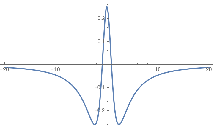
As t approaches ±∞, a approaches 0. This means that as t approaches ±∞, a hyperbolic spiral gets closer to Nielsen’s spiral (log-aesthetic curve with a=0).
In[]:=
Limit[alpha[t],t->Infinity]
Out[]=
0
In[]:=
Limit[alpha[t],t->-Infinity]
Out[]=
0
We can visualize how a changes depending on t . Note that at t=0, a hyperbolic spiral is not defined.
Plot[alpha[t],{t,-20,20},Exclusions->{t==0}]
Out[]=

Cite this as: Norimasa Yoshida, "Computing the slope of a logarithmic curvature graph" from the Notebook Archive (2024), https://notebookarchive.org/2024-06-1ucl8i6
Download
